Southern resident line up. (credit: Center for Whale Research)
A couple years ago Val put a bunch of effort into stabilizing a video of some rare southern resident killer whale behavior that Beam Reach observed during our first field program in fall, 2005. In support of an upcoming fundraiser for The Whale Museum, we have uploaded the stabilized version to YouTube and then stabilized it as second time using YouTube’s editing enhancement. (The original, shaky footage is also stabilized as of 2014, but only using the secondary YouTube stabilization.)
We hope the double-stabilized version (embedded below) doesn’t make you too seasick. You may also enjoy the links below and appended background information re-posted from what was originally published at orcasphere.net.
Stabilized video
Video credits go to Beam Reach students Brett Becker and Courtney Kneipp. Still photo credits go to the Washington State Department of Ecology and Iris Hesse of the Center for Whale Research. Listen for a very unusual simultaneous call made by many individuals during the last minute of the recording.
One of the most remarkable behaviors of the southern residents is the “greeting ceremony†in which two groups of orcas line up facing each other and then mingle together. This article describes a similar “ceremony†acoustically and visually (video; photo gallery), and then discusses whether it may have been related to a “greeting,†a “goodbye,†or a more complex combination of activities.
I offer it here in the hope that others who witnessed this particular event may further consider what occurred. Please feel free to comment on this article and/or contribute your thoughts via the discussion forum. Insights from other accounts of different “ceremonies†performed by the southern resident (or other) orcas would also be welcome. Perhaps we will piece together a publishable story?
On October 4, 2005, only a week into a month of sailing with the southern residents, students and teachers of the Beam Reach marine science and sustainability school approached San Juan Island along with members of J and L pods. The Beam Reach research vessel, the sailing catamaran Gato Verde, paralleled the orcas as they moved northward from Salmon Bank along the west side of San Juan Island during the mid-afternoon. In the early evening, starting around 4:30pm PST, the pods began to concentrate within 100 meters of shore below Hannah Heights.
The “ceremony†that we observed (along with Tom McMillen, observers from the Center for Whale Research, and Sharon Grace [and others?]) was similar to “greeting ceremonies†that sometimes occur in the spring as the southern residents return to the Salish Sea from their winter ranges. One group of at least 9 adults and one calf (probably a subset of the group that had been traveling northward with us) congregated within 100 meters of shore ~0.5km southeast of a promontory with abundant driftwood (48o 29.65N, 123o 7.62W). They remained on the surface, gathered into an extremely tight group, traversed the shoreline southward for a few minutes, then doubled back to the north. Meanwhile, a different group of at least 9 adults rounded the driftwood point, heading south, and began to congregate in a rough line just south of the promontory’s rocky bluffs. They, too, remained largely on the surface, drew together in a line, and proceeded slowly southeastward toward the southern group. When they were about 25m apart, the southern group lunged forward, submerged, and quickly met the northern group. The two groups mingled, turning quickly and making brief dives, and remained together for an extended period (at least 15 minutes — we left at ~5:15pm to make port before nightfall — and probably much longer).
The ceremony was documented by Beam Reach with still photographs, digital video, and stereo underwater sound recordings. Preliminary analysis of the still photographs and video suggests that at least J40, J14, and L41 were part of the southern group. Tom McMillen of Salish Sea Charters with Iris Hesse and EEH (??) of the Center for Whale Research (CWR) were drifting near the northern group and photo-identified many of its members. Based on an initial examination of still photographs taken of the combined groups, Dave Ellifrit of the CWR noted that L84, L41, L90, L72, L55, L82+calf, L25 with L41, and Raggedy (K40) were present. Any additional photo-identification (and associated) debate is welcome!
An interesting aspect of this event, first pondered by Tom McMillen (and later discussed with Ken Balcomb and Dave Ellifrit?), is that it approximately coincided with the last time that the matriarch L32 was seen. Earlier in the day (about an hour before the ceremony began?), Tom observed L32 with son L87 and noticed that she was emaciated and had a weaker-than-normal blow. CWR photographs confirm that L32 had a sunken blowhole area (“peanut headâ€) that day. L32 was not observed after the ceremony and L87 was observed the next day (or maybe 2 days later?) without L32, so L32 is now presumed to be dead. Could we have witnessed a “goodbye†ceremony?
Perhaps, but the CWR photographs reveal that the ceremony also involved foraging (birds hovering over orcas at surface) and sexual activity (sea snakes). Beam Reach video shows traveling behavior, milling, tail lobs, and pectoral fin slaps. There was a lot of acoustic activity prior to the meeting of the two groups, including abundant echolocating and intermittent calls, and an amazing coordinated acoustic event in which many individuals call simultaneously (without an obvious cue).
I’ve created this movie that juxtaposes the best of the Beam Reach video and underwater sound. Please note, however, that I was unable to synchronize the sound and video. I am tempted to associate the simultaneous calls with the dynamic lunge of the two groups together, but (I regret) there is currently no way to know whether that is right. Video footage was acquired by Beam Reach students Brett Becker and Courtney Kneipp. Acoustic data is from 2 ITC hydrophones mounted 1.4m apart on a horizontal pipe at 4.4m depth. (The engine noise at the beginning of the movie is from the Beam Reach research vessel.)
Please don’t hesitate to comment, email, or start a discussion thread if you have information or ideas about this fascinating behavior of the southern residents.
Notes by an oceanographer from an upper trophic (orca) perspective during the outer-coast/less-local/more-regional portion of the annual meeting of the Marine Waters Monitoring Workgroup of the Puget Sound Ecosystem Monitoring Group (PSEMP) at APL/UW on 3/28/14. This meeting is a rare effort and opportunity to synthesize ocean observations from the previous year and across the Salish Sea and outer coast of the Pacific Northwest region (with an over-emphasis on Puget Sound). I was not able to stay for the rapid-fire talks related to plankton & pathogens (e.g. harmful algal blooms) or water quality.
Freshwater inputs — Ken Dzinbal
In long-term medians from rivers across region, the overall long-term seasonal pattern is a dry period in Sep-Oct (extending into late fall for some rivers), then a wet spring with big storm pulses Feb-June. In 2013, Fraser mean daily discharge at Hope (above tidal influence) peaked in late May, ~1 month earlier than historic median.
Fred Felleman mentioned that 2013 was a terrible year for Fraser river Chinook and a bumber year for Columbia Chinook, and that the Southern Resident Killer Whales (SRKWs) responded one would expect for the “best salmon samplers on the planet” — they were rarely sighted in inland waters and tracked often on the outer coast near the Columbia river mouth. PSC Fraser panel is a good source of historic data on Fraser flows.
Boundary conditions & water masses — Skip Albertson
Less upwelling in Aug/Sep; SW winds! Usually we have N winds and upwelling in September, but we almost had down-welling due to unusual winds out of the southwest.
We looked at Pacific Decadal Oscillation (PDO), and index that changes slowly. Initially there was colder water up against the coast, but then offshore waters got warmer and warmer. Overall in 2013, the PDO index was slightly lower than long-term means.
Cha’ba mooring (offshore Washington) — John Mickett
Temperature-Salinity plot for all of Puget Sound shows median values near 11 oC and 30 psu with low (6.5 mg/l) dissolved oxygen (DO) levels. This suggests a stronger-than-usual influence of oceanic water. Christopher Krembs pointed out that the goal is to start looking at Puget Sound water properties in terms of water masses that may traverse the different basins, rather than
The big story on the outer coast in 2013 was the hypoxia. John showed pictures of many dead Dungeness crabs washed up on Ruby Beach. Looking at data from 3 and 84 meters, you see phytoplankton blooms (chlorophyll concentrations up ~20 micrograms/l). In mid-August we saw DO levels drop to ~1 ml/l a level which stresses or kills organisms. At about the same time we saw very unusual warm surface water temperatures (up to 16-18 oC, well above the long-term means of ~12 oC) which were due to the wind reversals that led to stratification and subsequent solar-heating.
Upwelling comes from 30-40m (ref Ryan McCabe) and has much higher DO than what we saw. That’s why we think these low DO events in the shallow water were advected horizontally, having formed somewhere else.
End of May (5/31) and beginning of July (7/1) sees Columbia River plumes in surface waters. Are these related to court-ordered dam releases?
San Juan channel — Jan Newton (slides from 2013 research apprentices)
North station off NE San Juan Island; South station just south of Cattle Pass (tends to picks up Pacific Ocean influence)
Normally, Fraser plume is advected south in the summer and north in the winter, with associated up-/down-welling changes. It creates a strong pycnocline near 30-40m.
Redfield AC (1950) Note on the circulation of a deep estuary: the Juan de Fuca-Georgia Straits
In 2013, TS plots from Centennial calibrated CTD show that 2012 was an anomalously cold year. The 2013 T-S ranges were +1 oC higher, and slightly fresher. In mid-October the cold 2012 water was ~0.5oC lower than long-term medians.
PDO shift from + to – values near 2007 correlates with warmer to cooler transition in inland water temperatures. There are initial hints that during the inland cooler periods we see higher seabird (and other upper trophic level animal?) populations.
CPODs and land-based visual observations. CPODS for 3 years in Burrows Pass, also at Biz Point and now at PTMSC
Harbor porpoise population plummeted in 50s, were nearly gone in 70s and now seem to be on a rebound.
Acoustic detections from Burrows typically show nighttime peaks of ~50 minutes/hour and 1/10th those levels during the day.
Click rates of 400-600 clicks/s during foraging; about 20 clicks/s otherwise (histogram).
Seasonally they are less present during the summer (low in May/June) than winter at Burrows Pass (based on visual sightings).
Primary prey is herring, smelt, and sand lance. Florian Granger (did PhD in Europe on harbor porpoises) says that they often travel in groups of 3.
What about anchovies and the possible decadal dynamics on the outer coast?
John Mickett asked why the diurnal pattern is so strong in Burrows Pass. Aileen thought that they were targeting animals that follow the vertical migration of zooplankton to surface waters at night, but also suggested day-time boat interference might be a factor (but implied they had not quantified boat traffic). Dzinbal suggested that squid might be following the zooplankton…
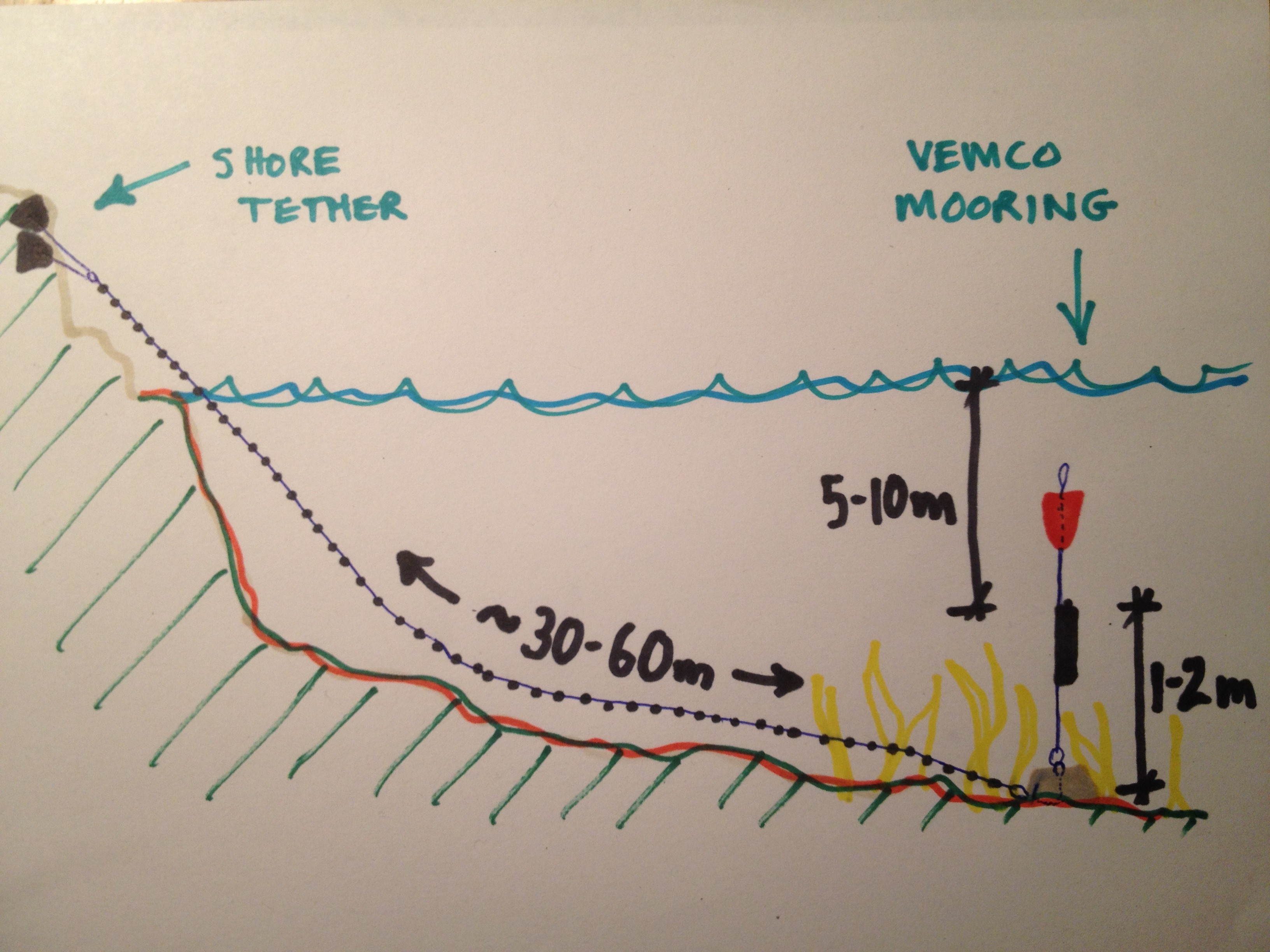
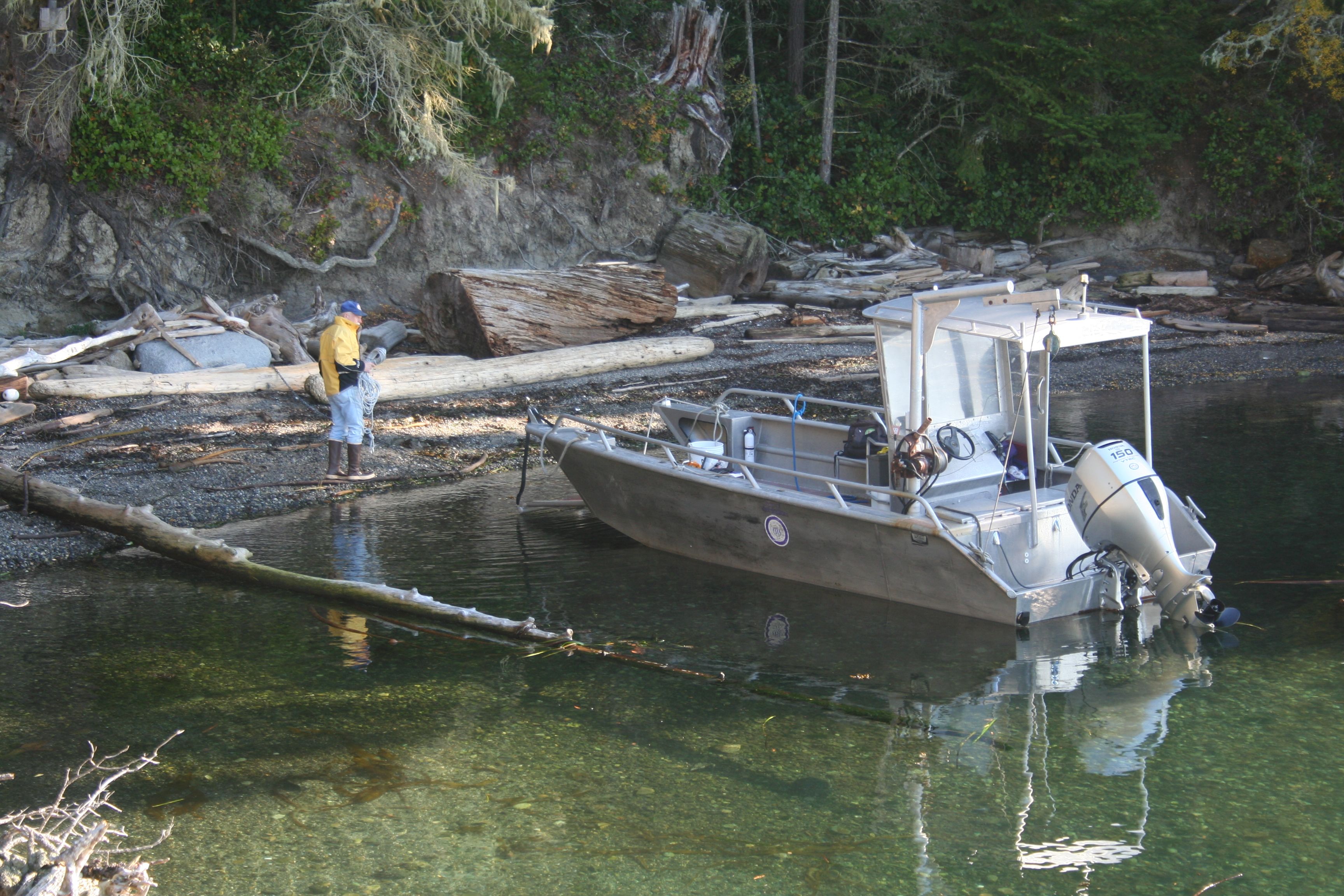
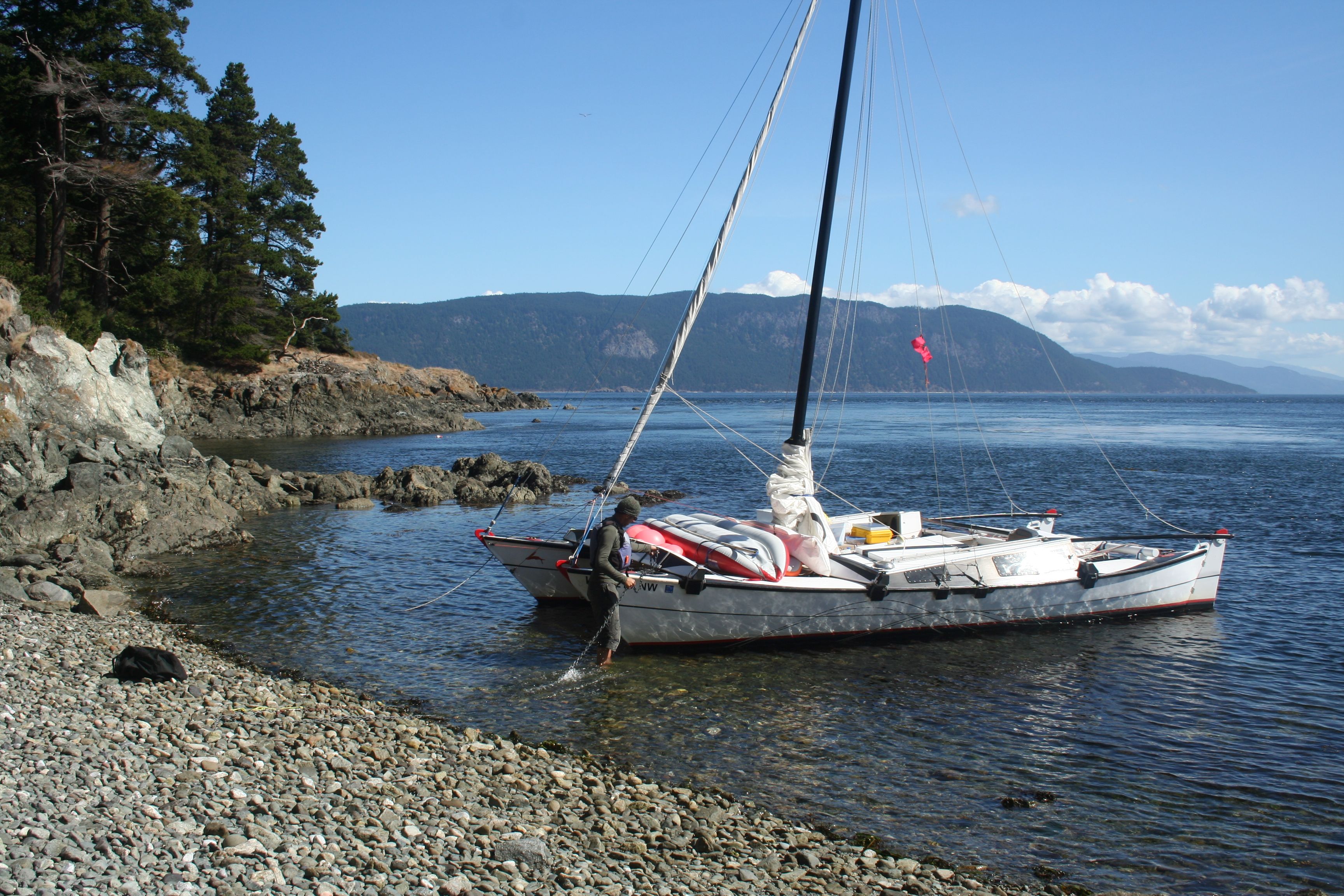
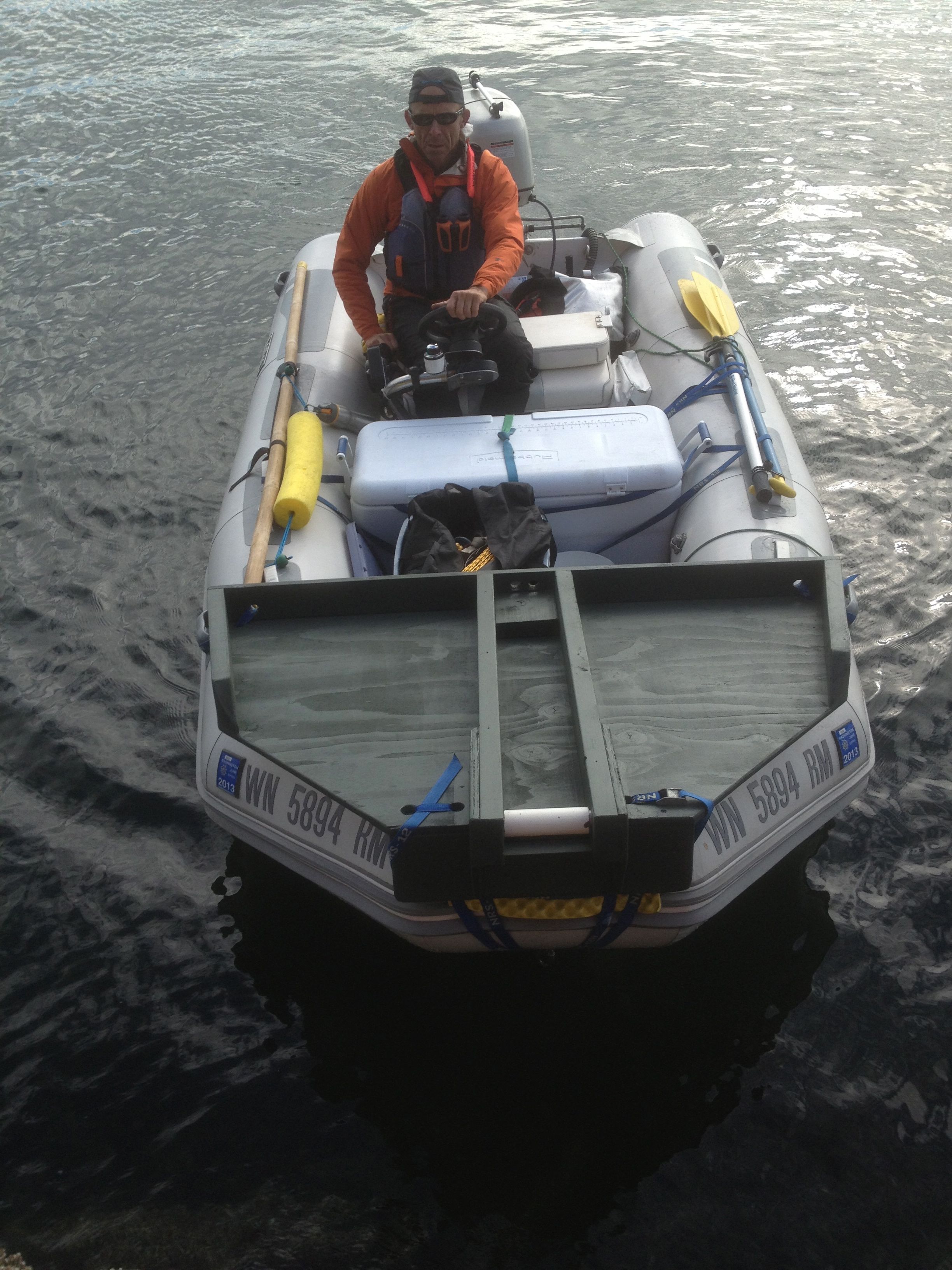
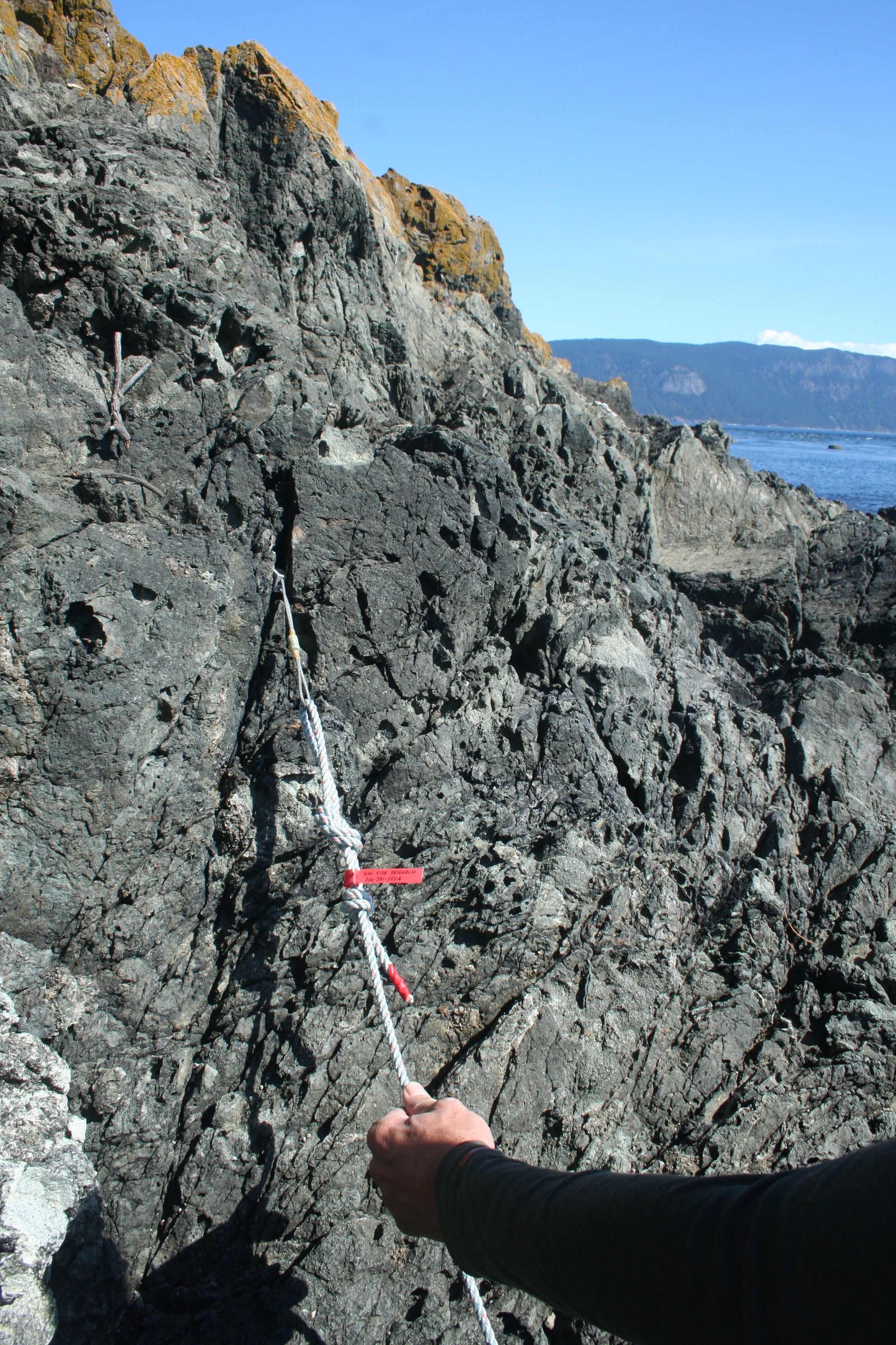
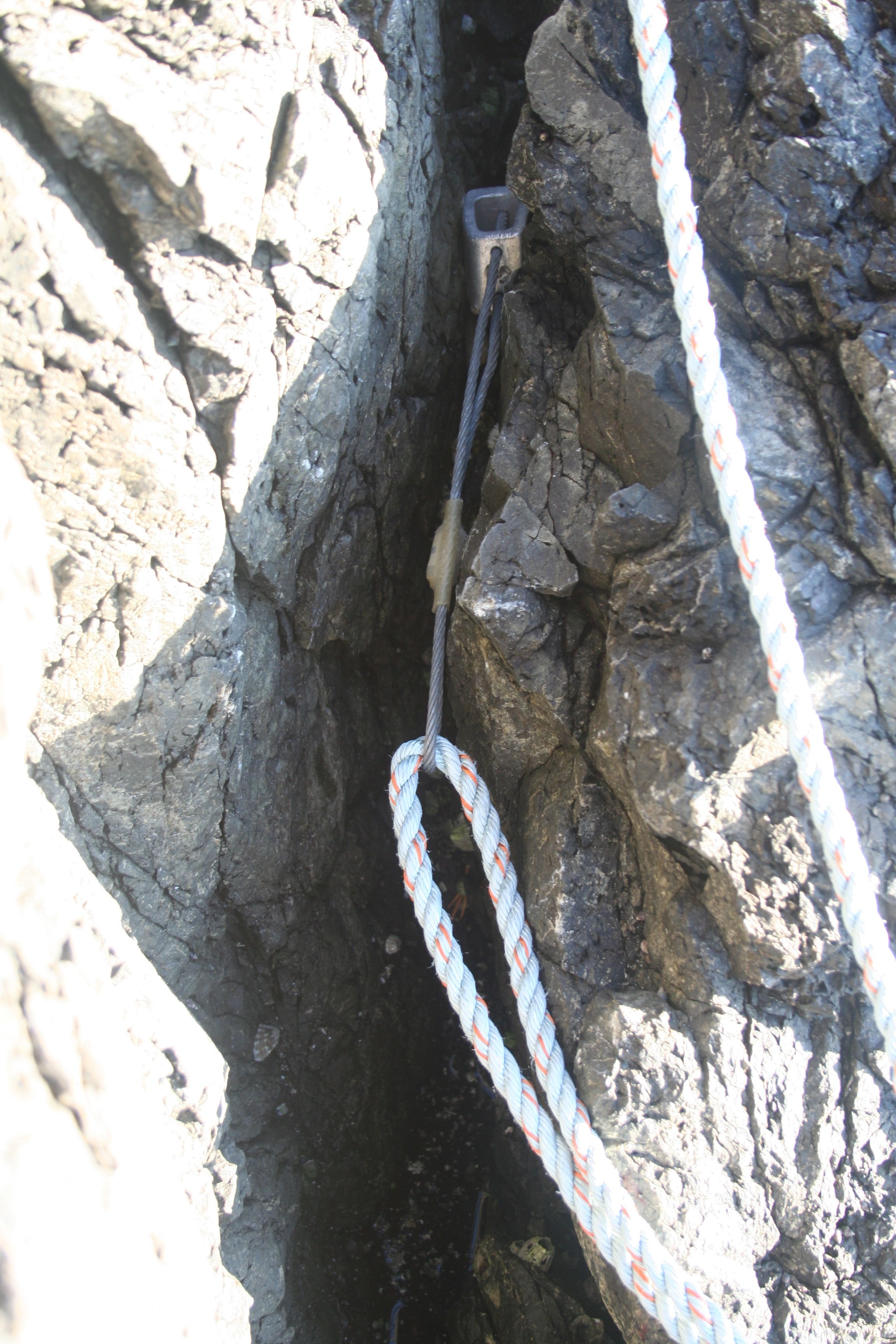
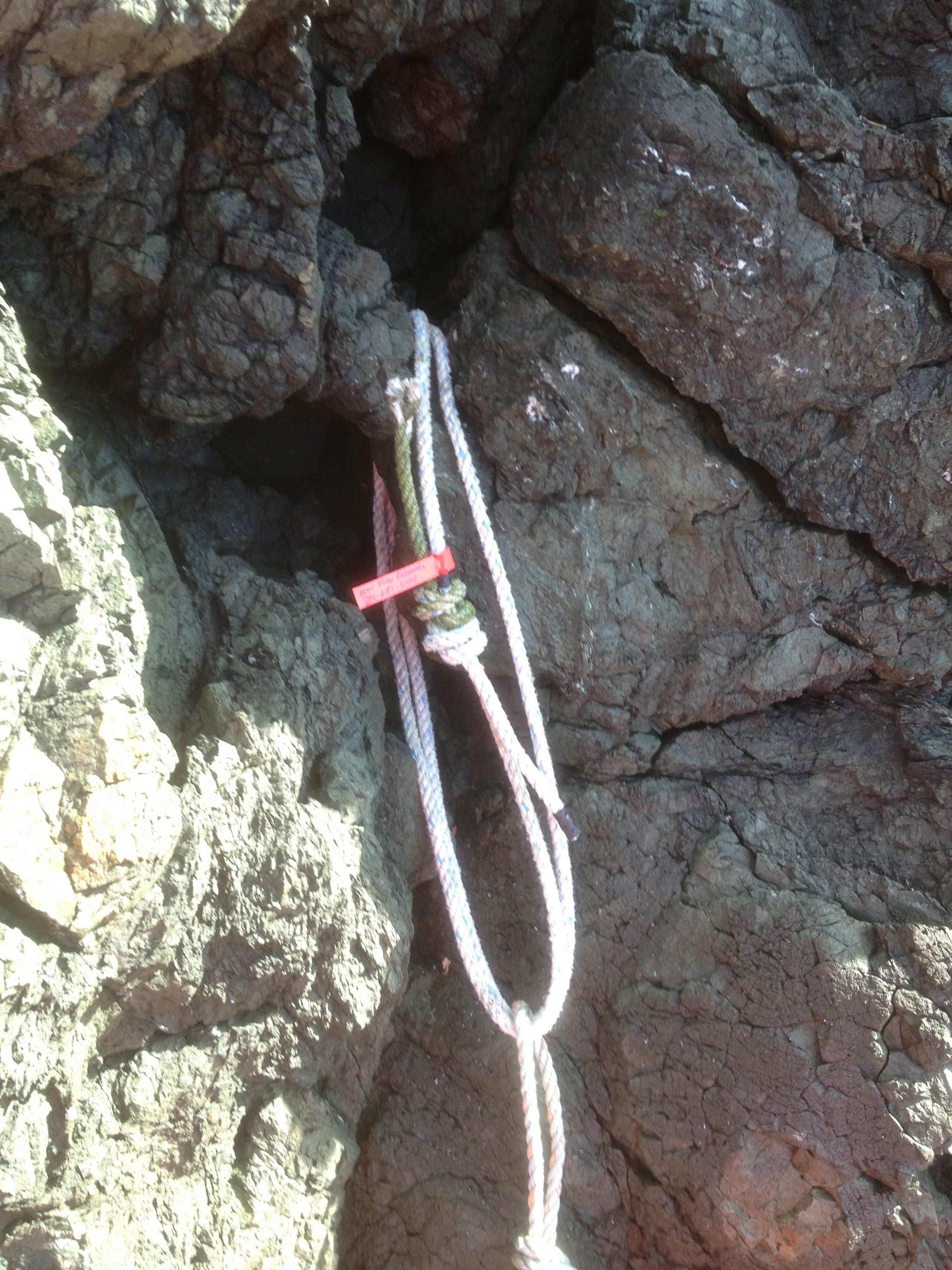
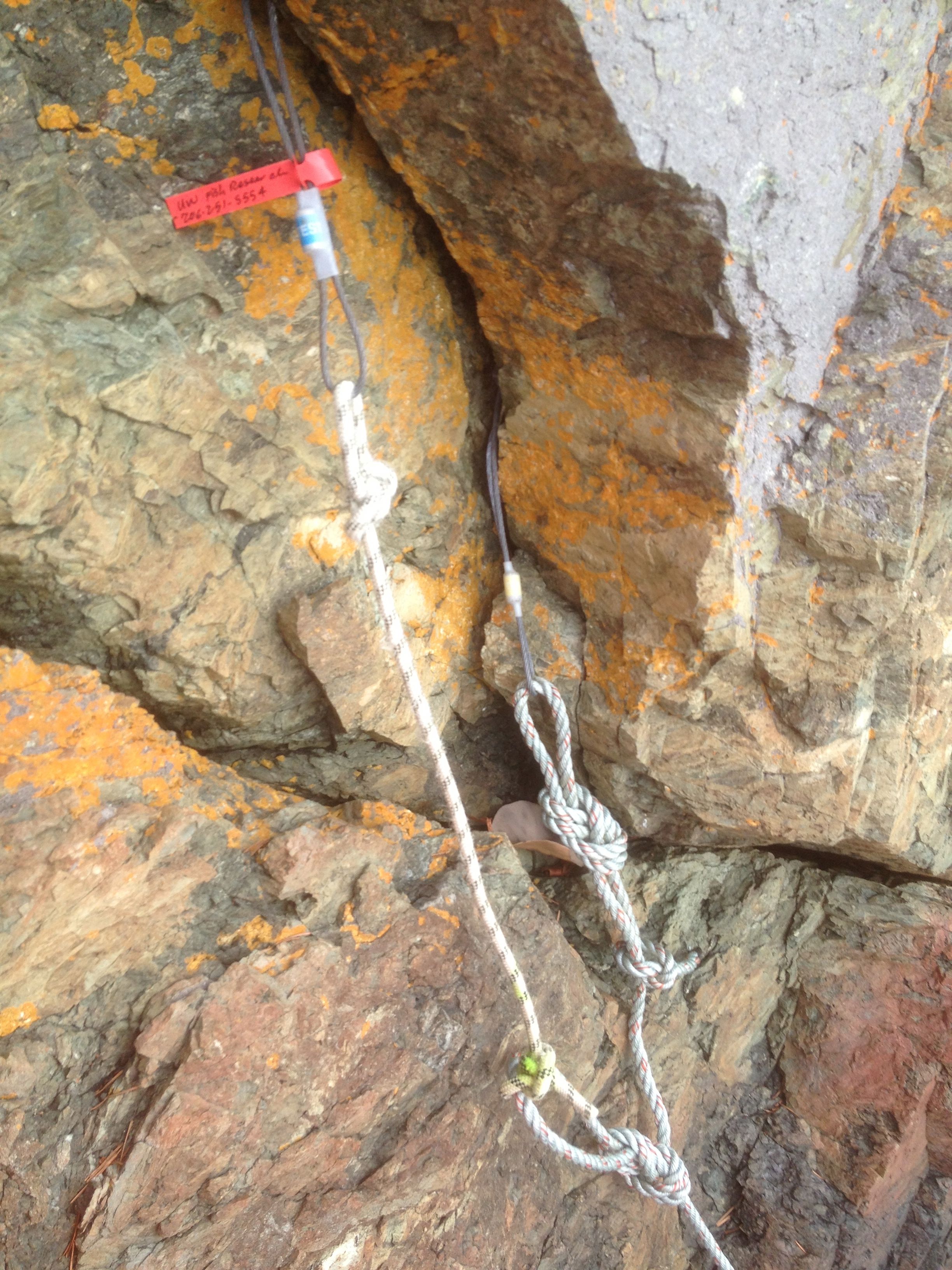
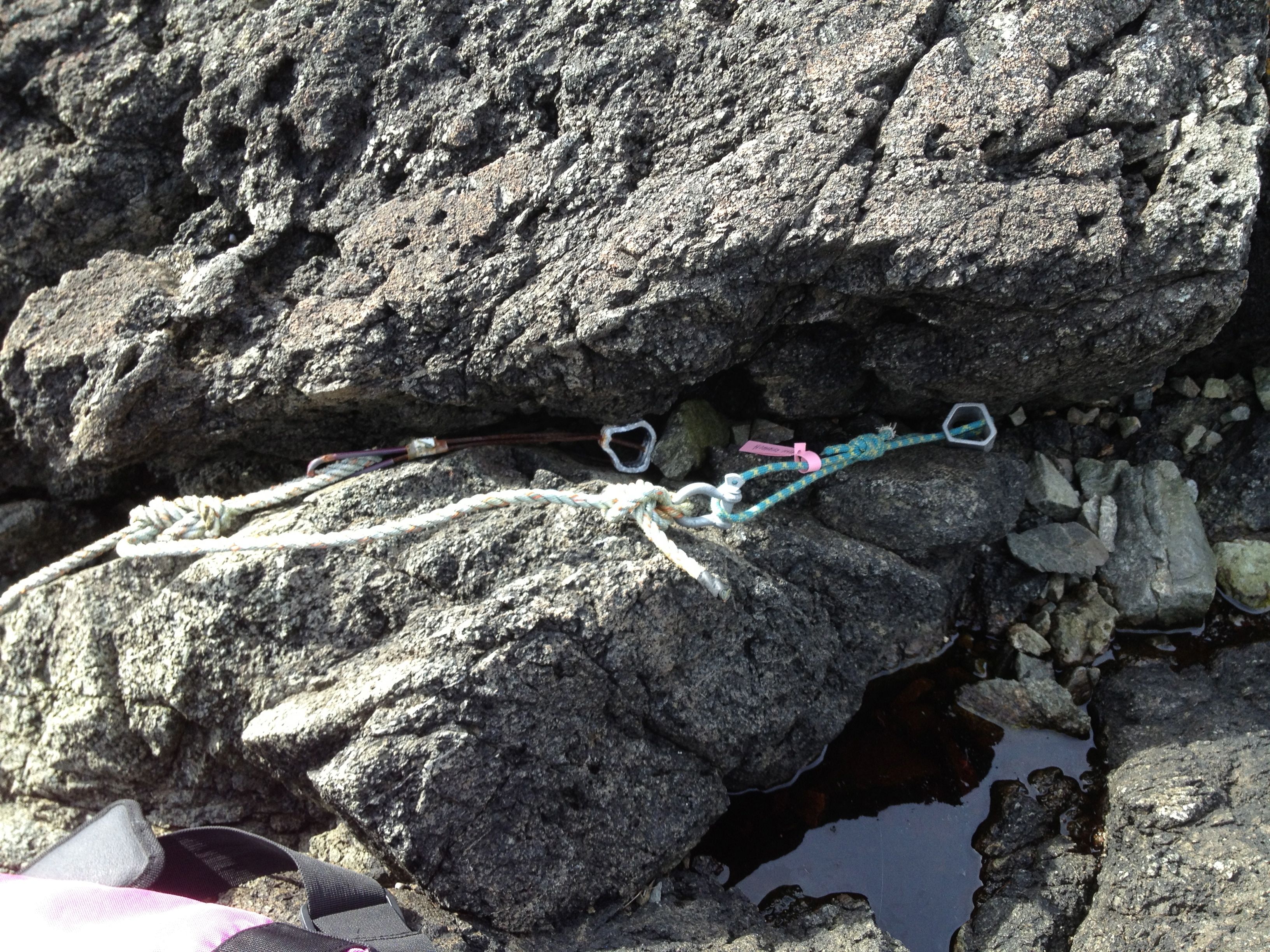
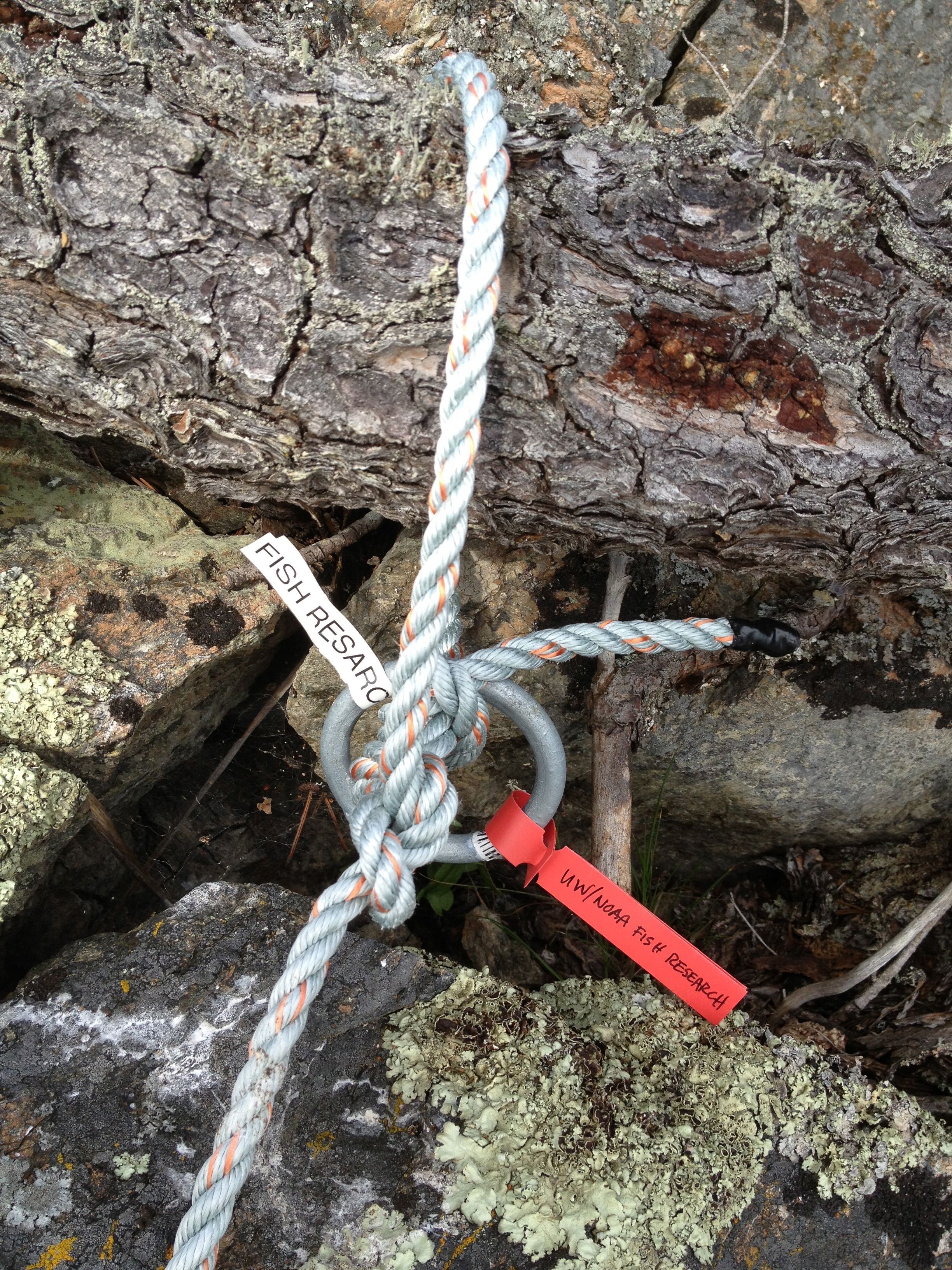
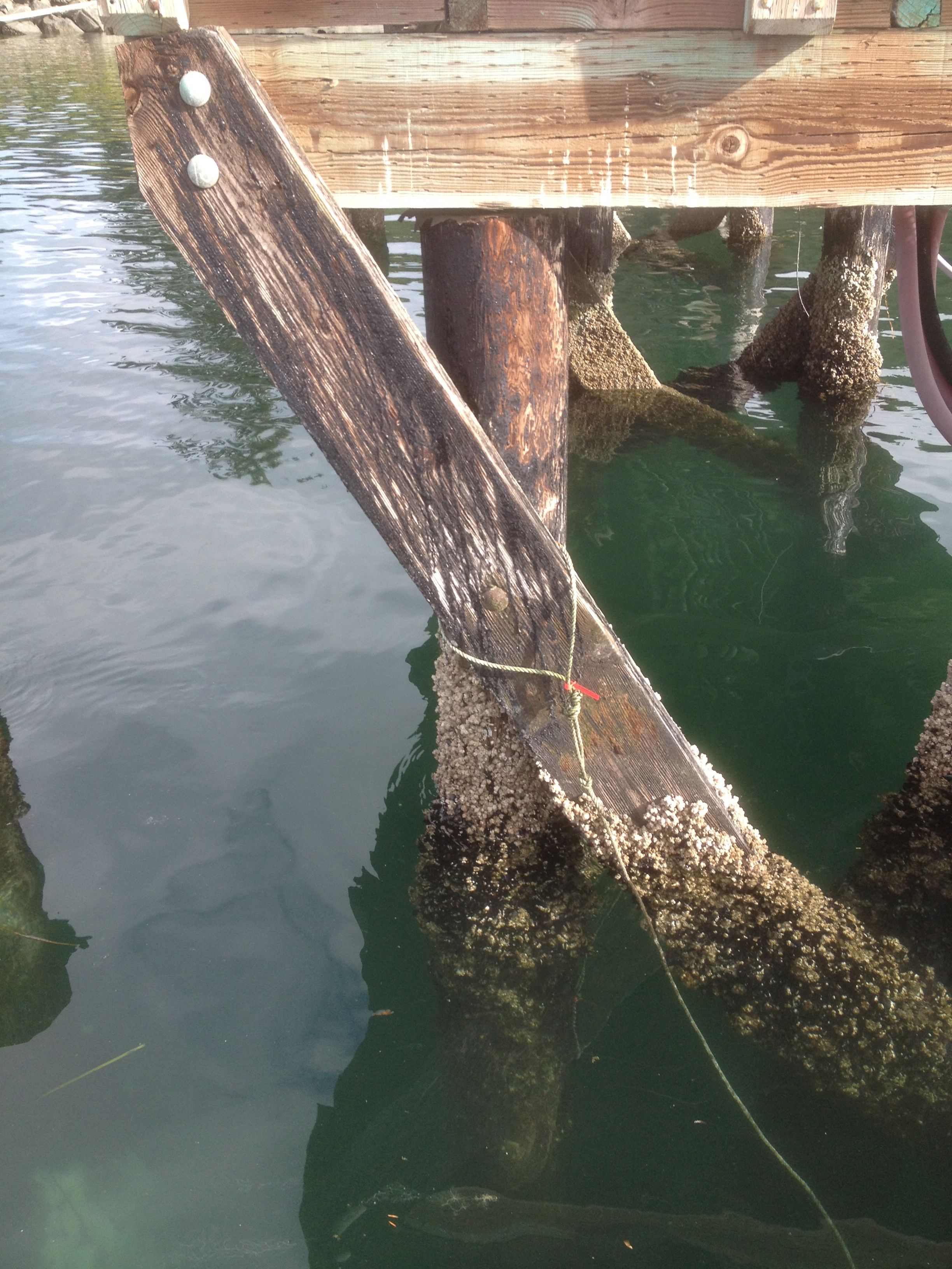
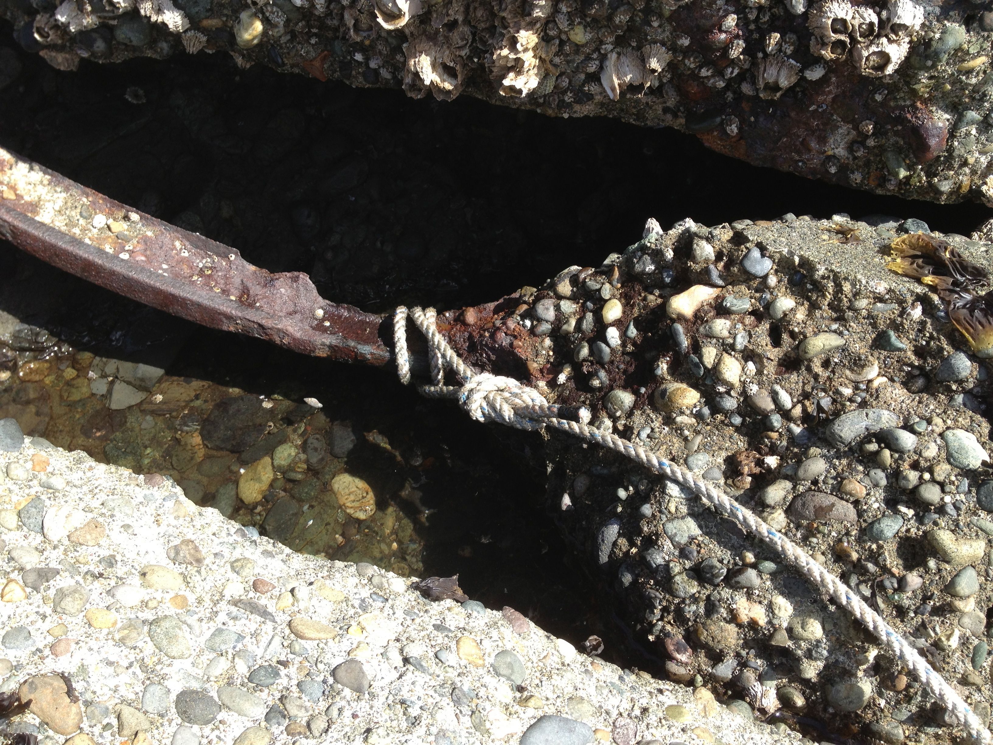
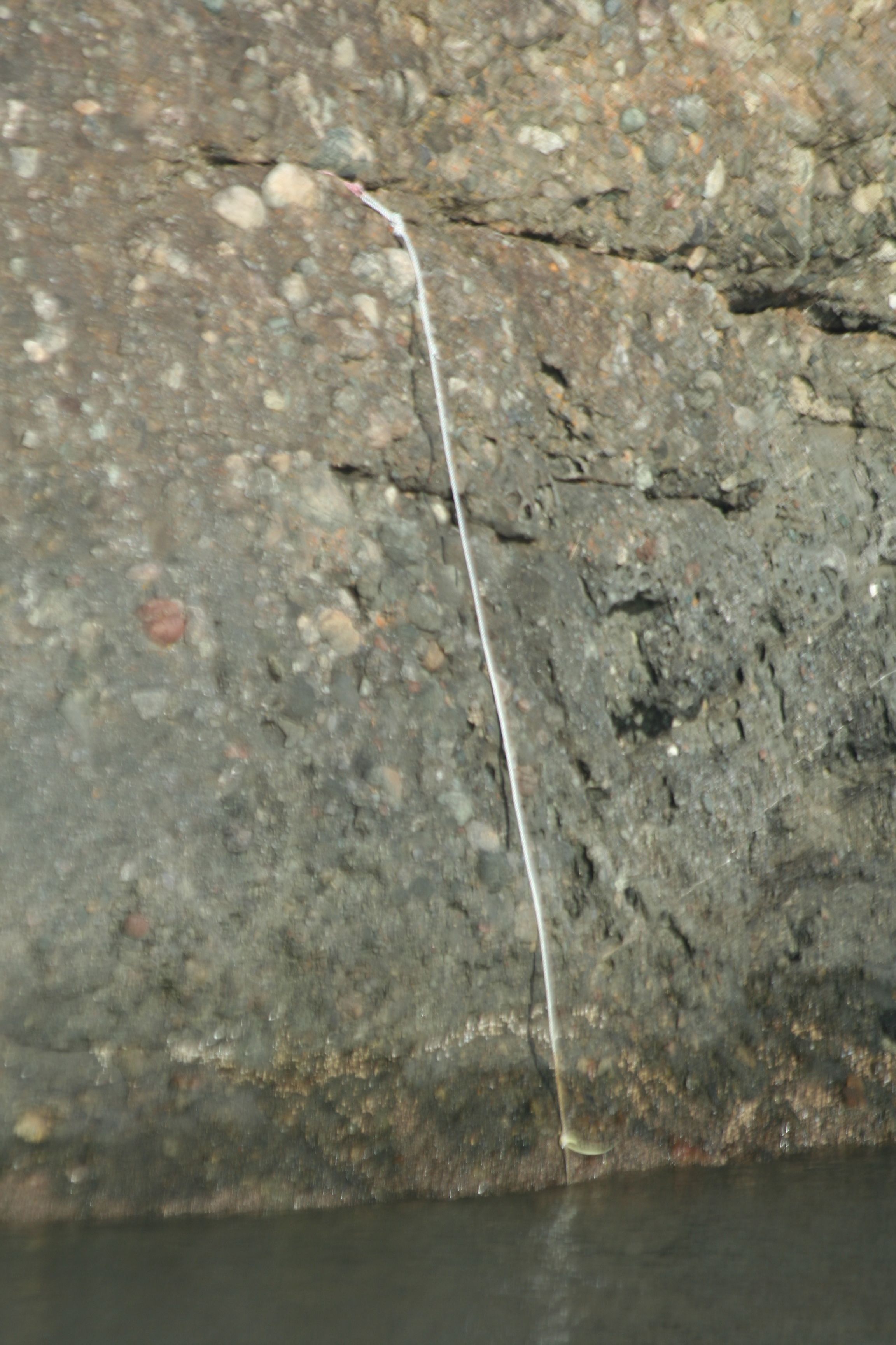
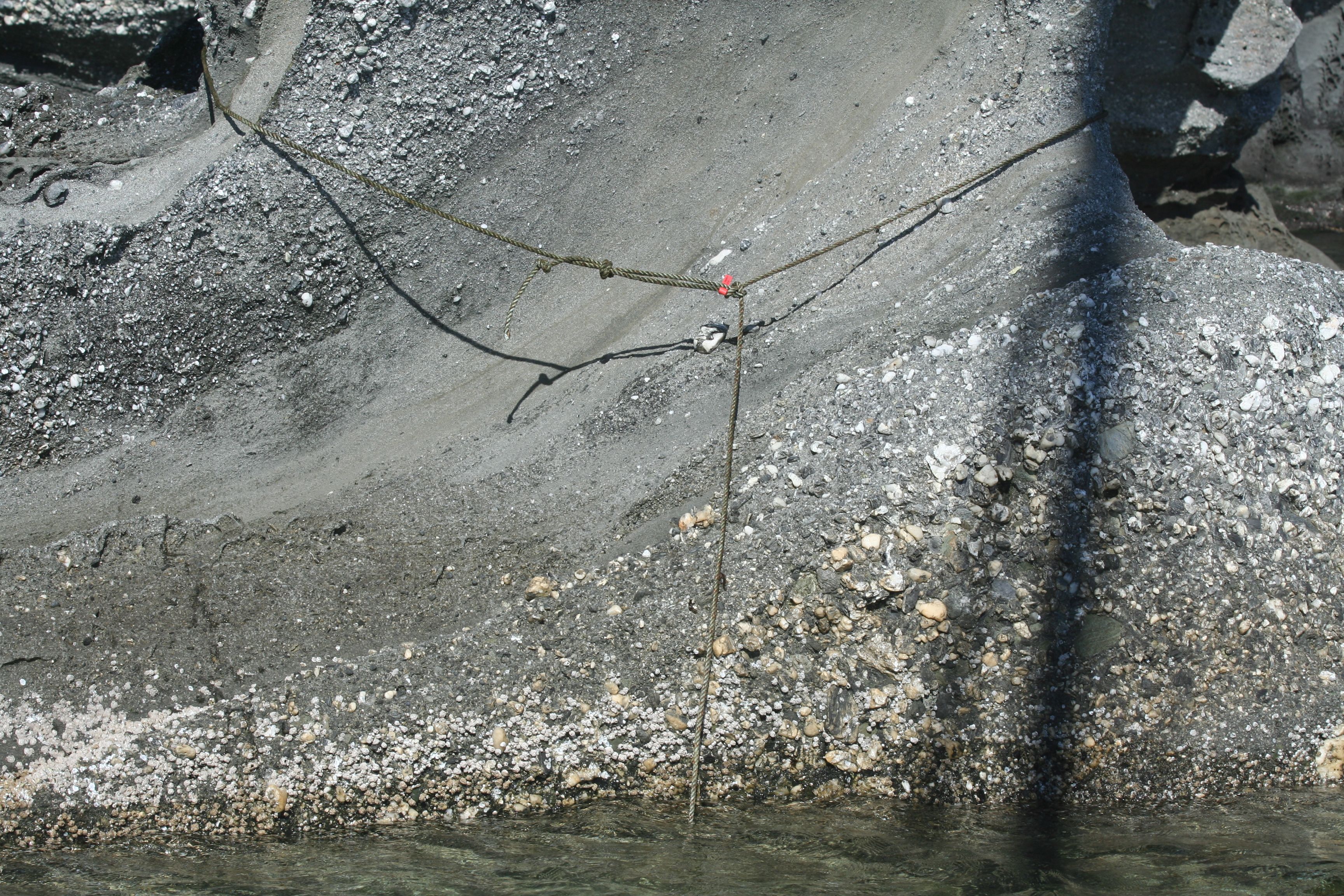
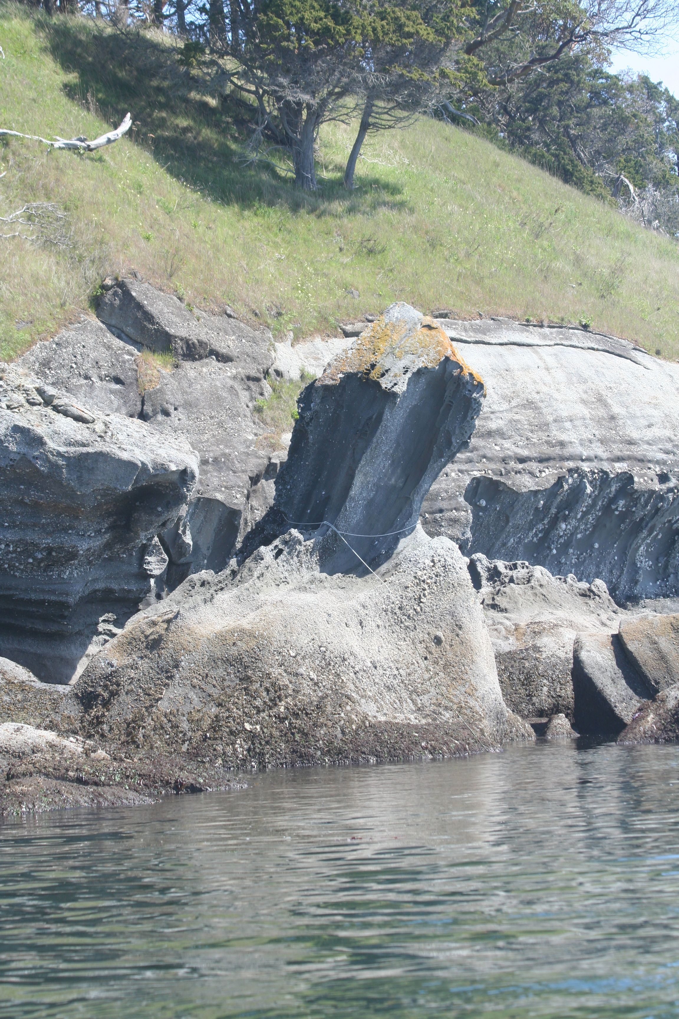
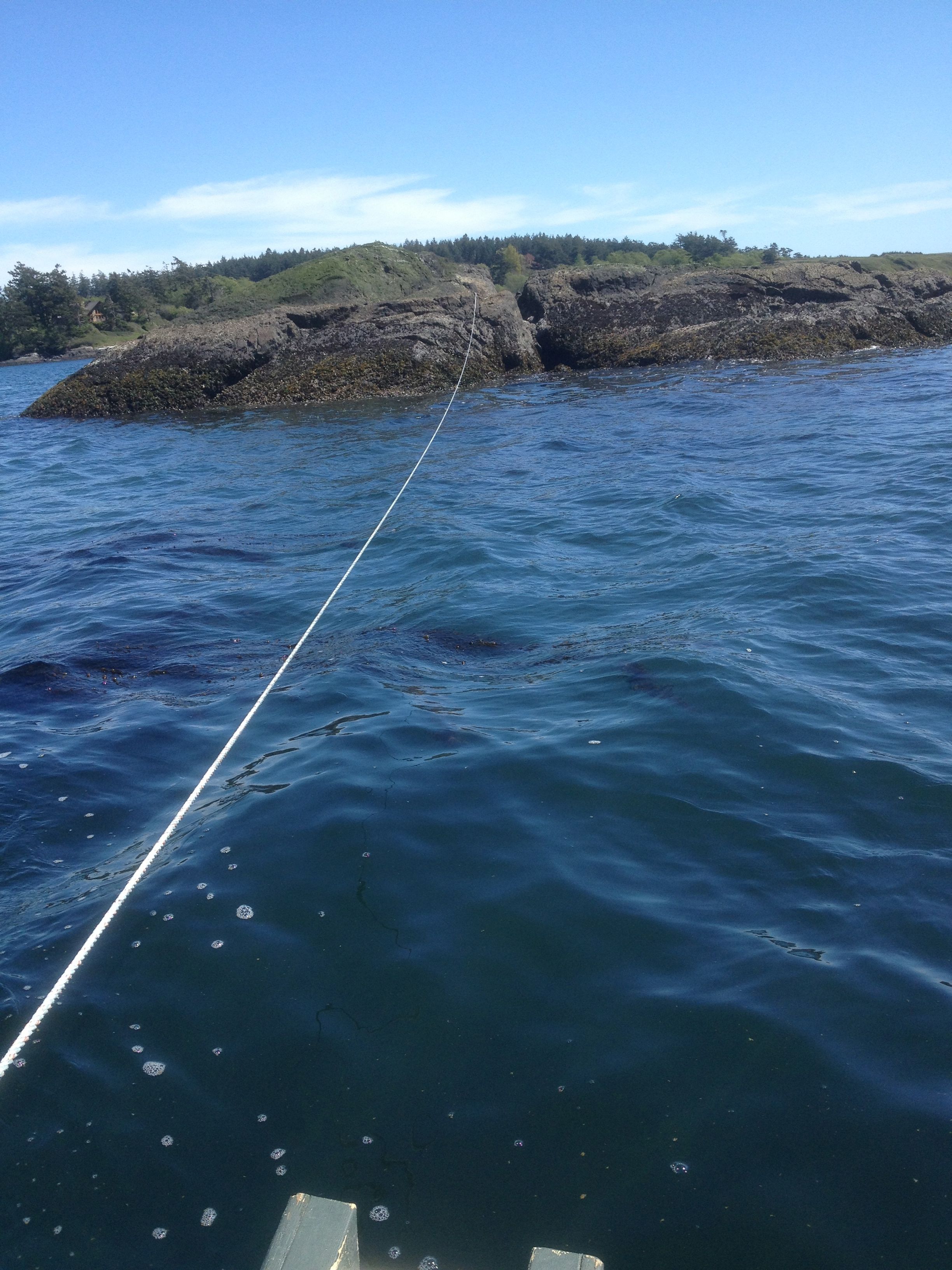
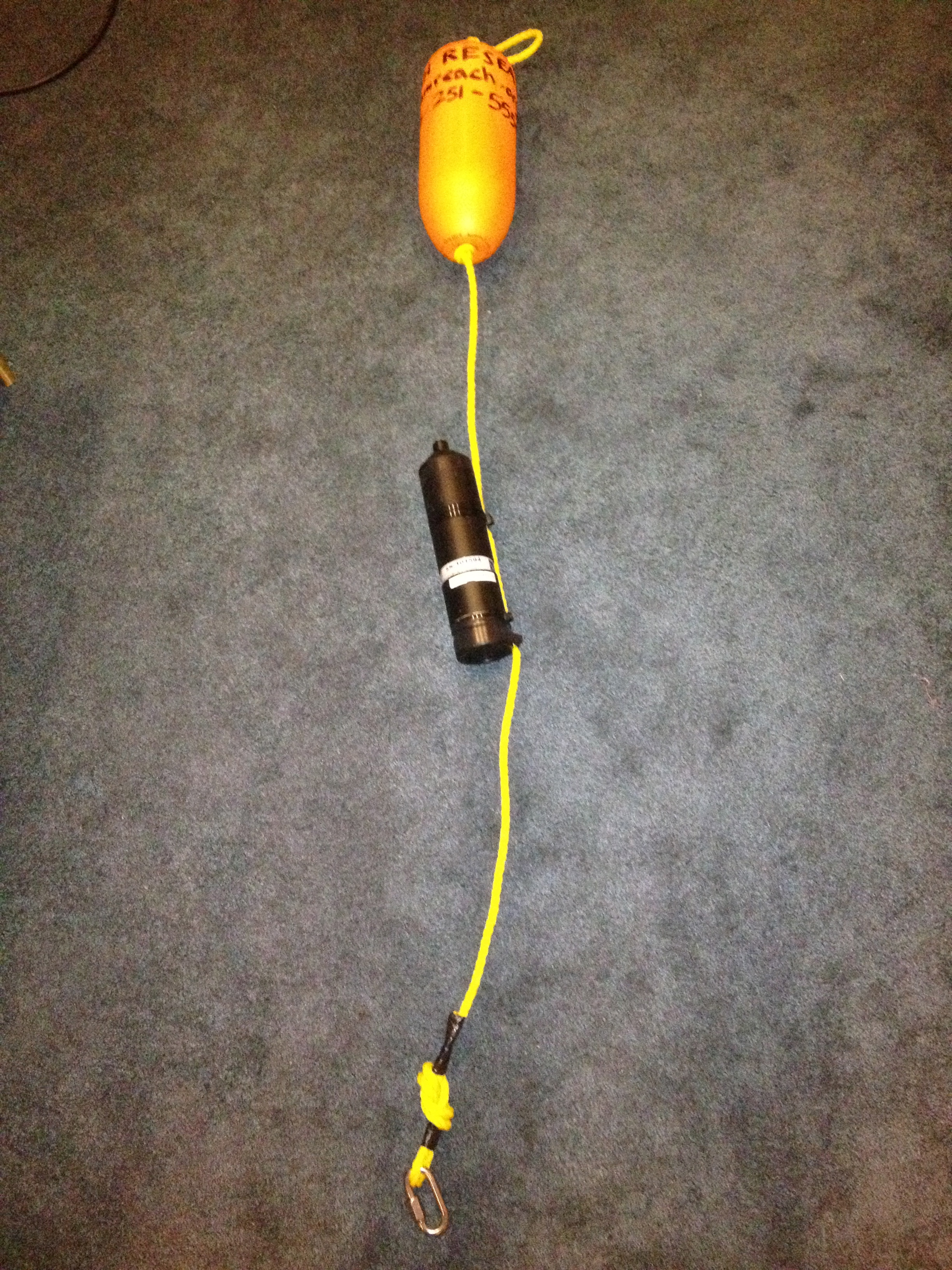
During our study of adult salmon movements in the San Juan Islands, we tested a novel method of deploying Vemco (VR2W) receivers. With permission from local land-owners, we used free climbing equipment or pitons to anchor a crab pot line to the rocky shoreline, marked it as fish research to discourage vandalism or theft, and then used it to tether the Vemco receiver mooring to shore. This allowed us to deploy and recover the mooring from a small boat, saving the cost of divers and simplifying the re-location of a mooring.
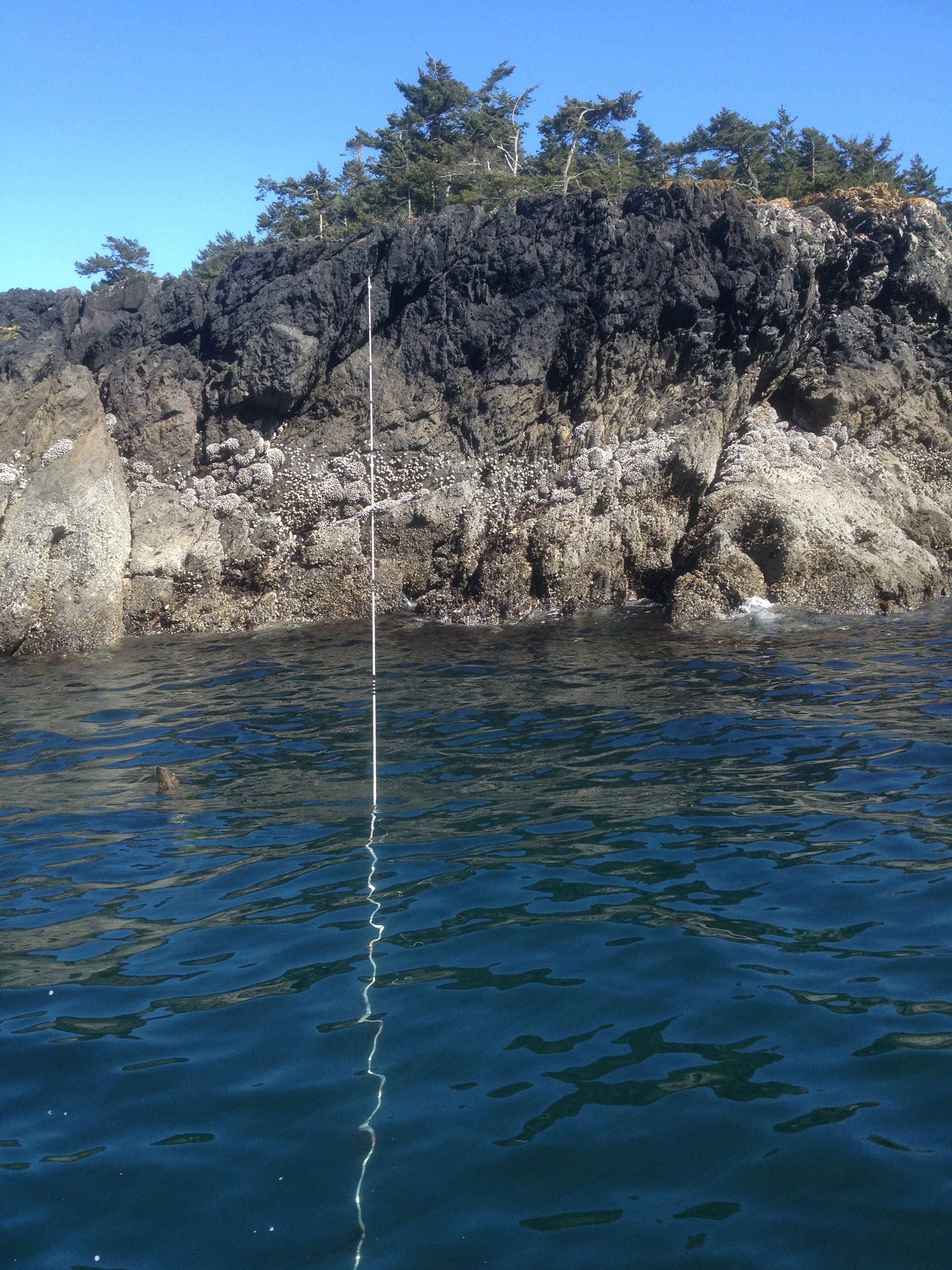
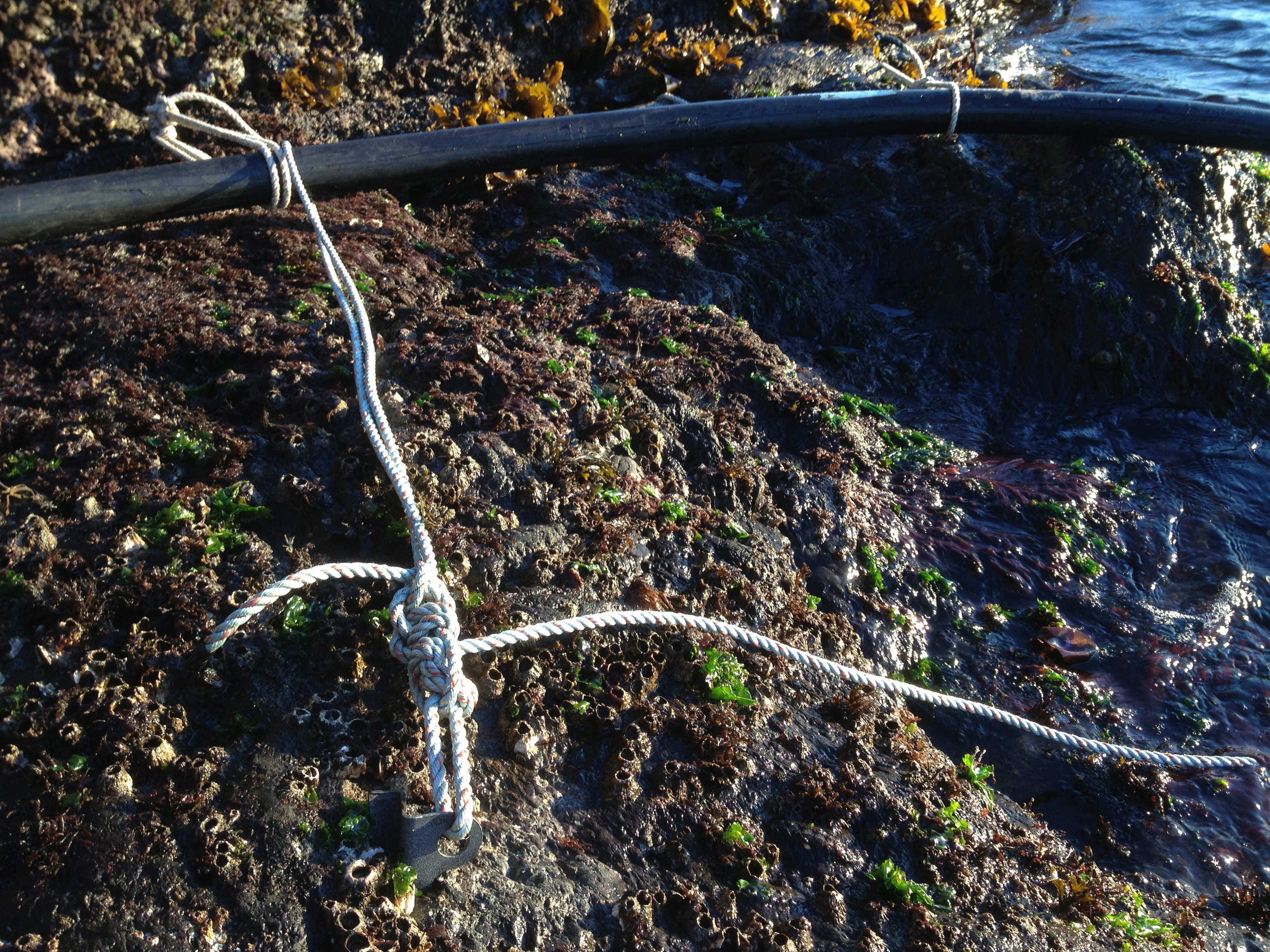
Schematic of shore tether method
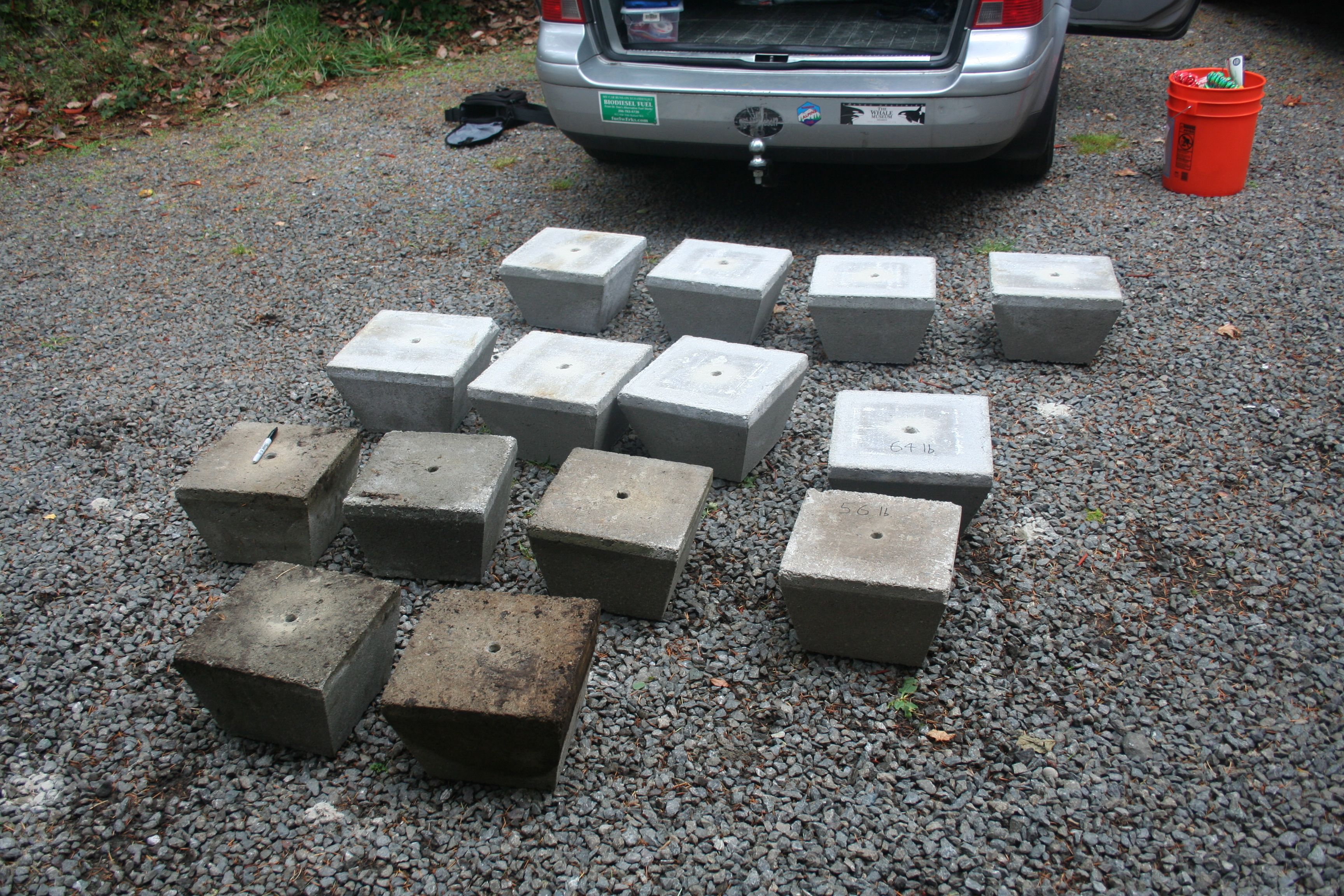
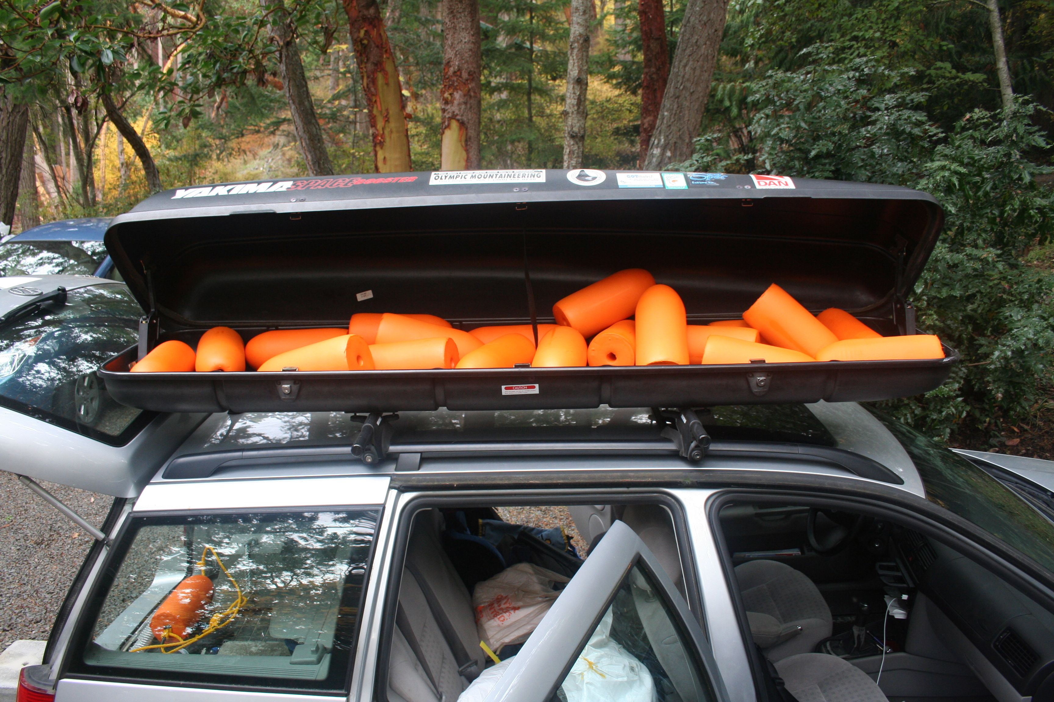
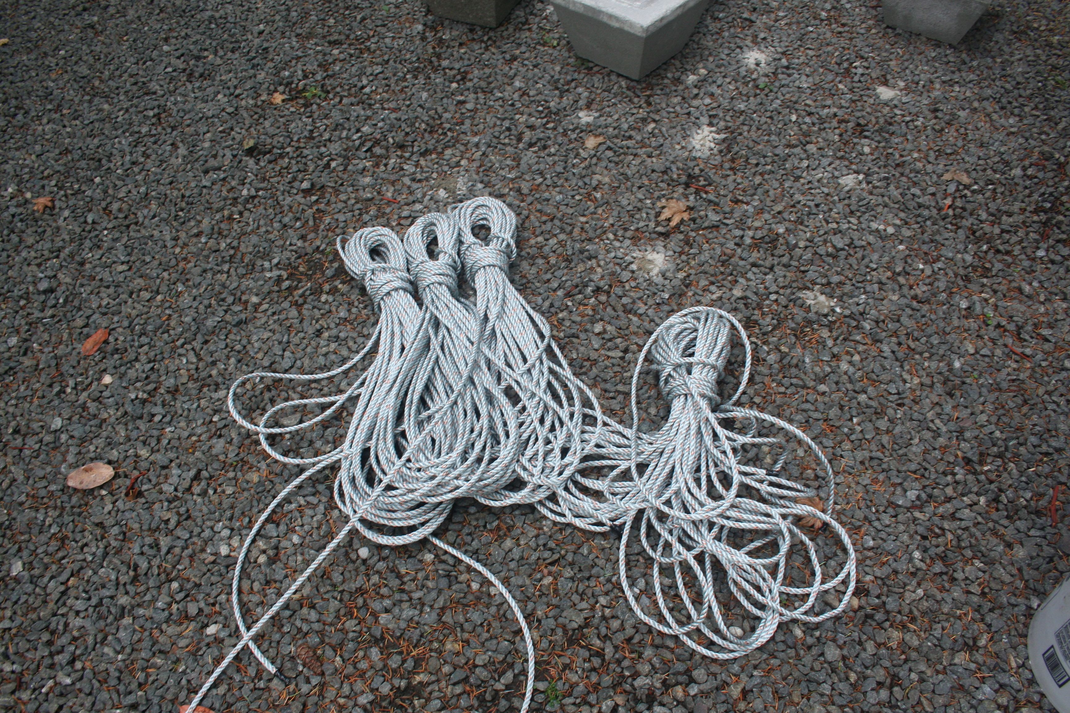
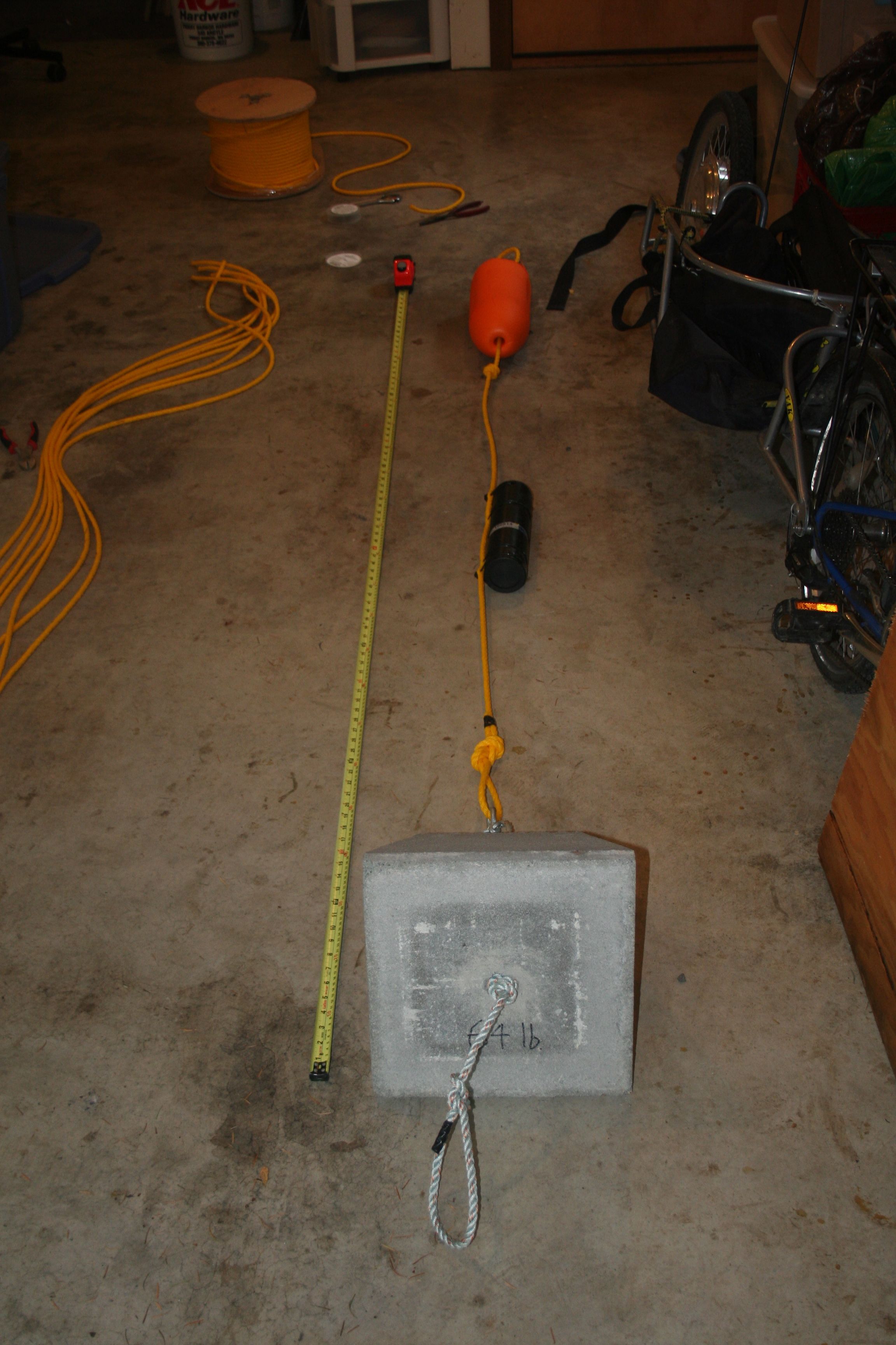
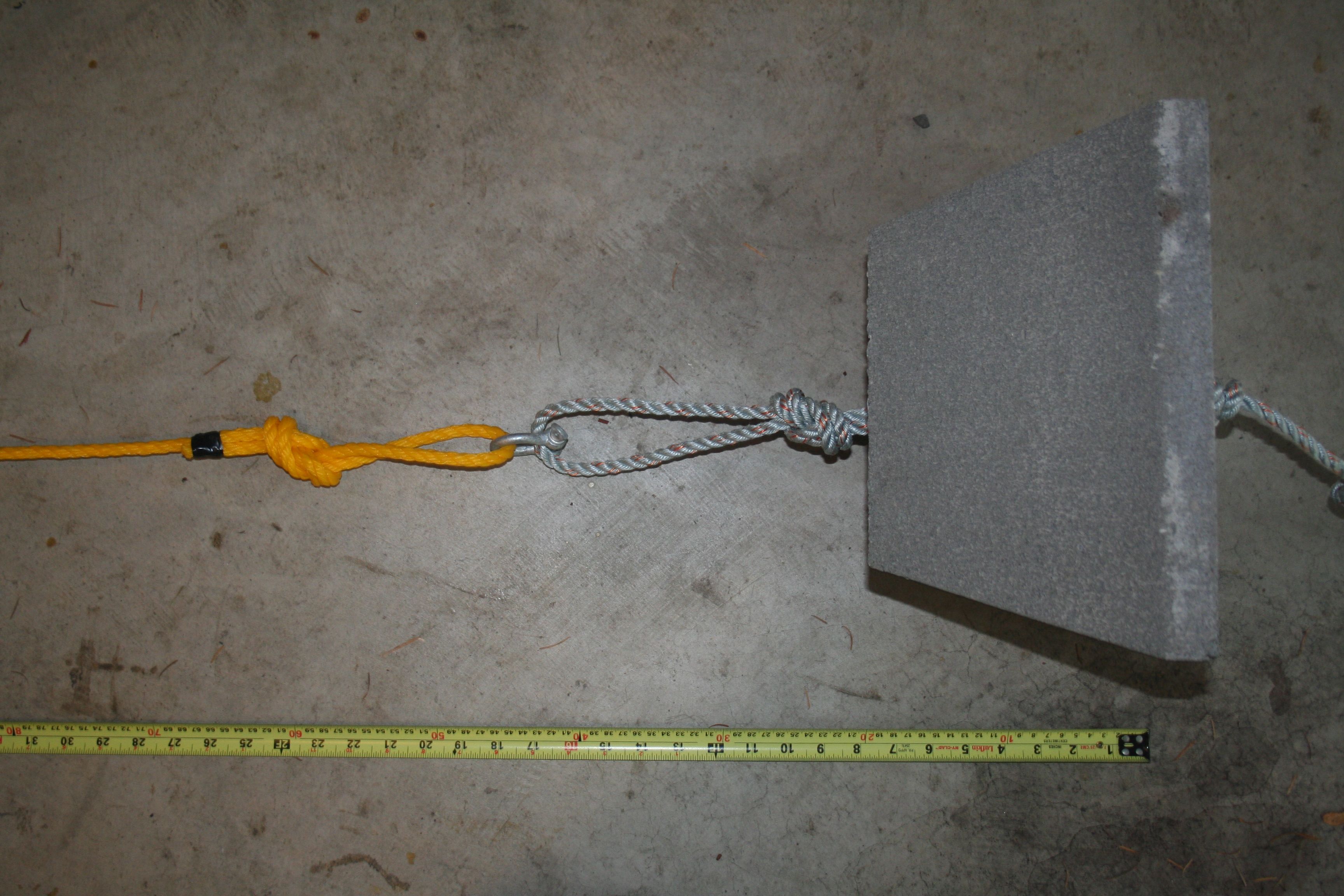
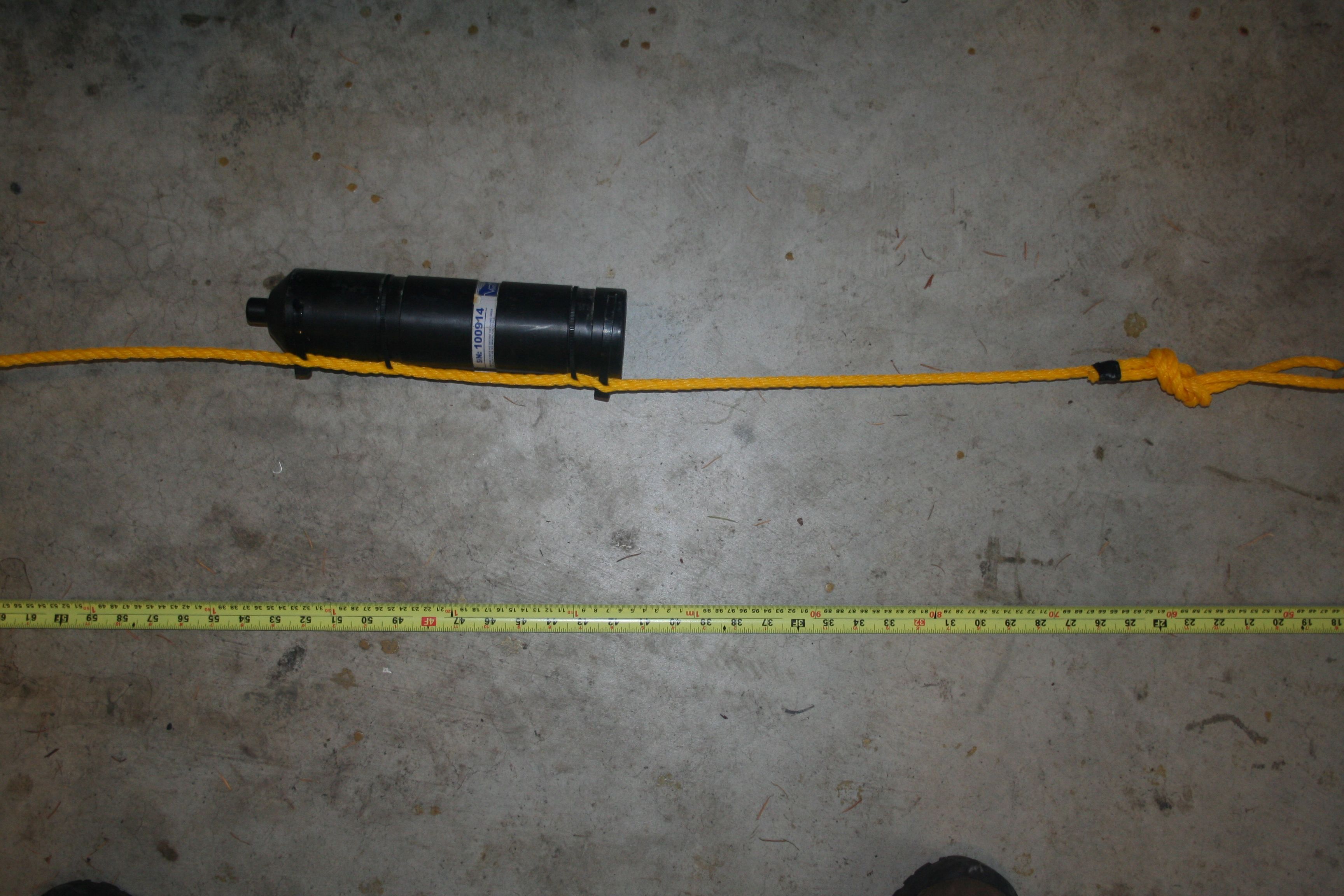
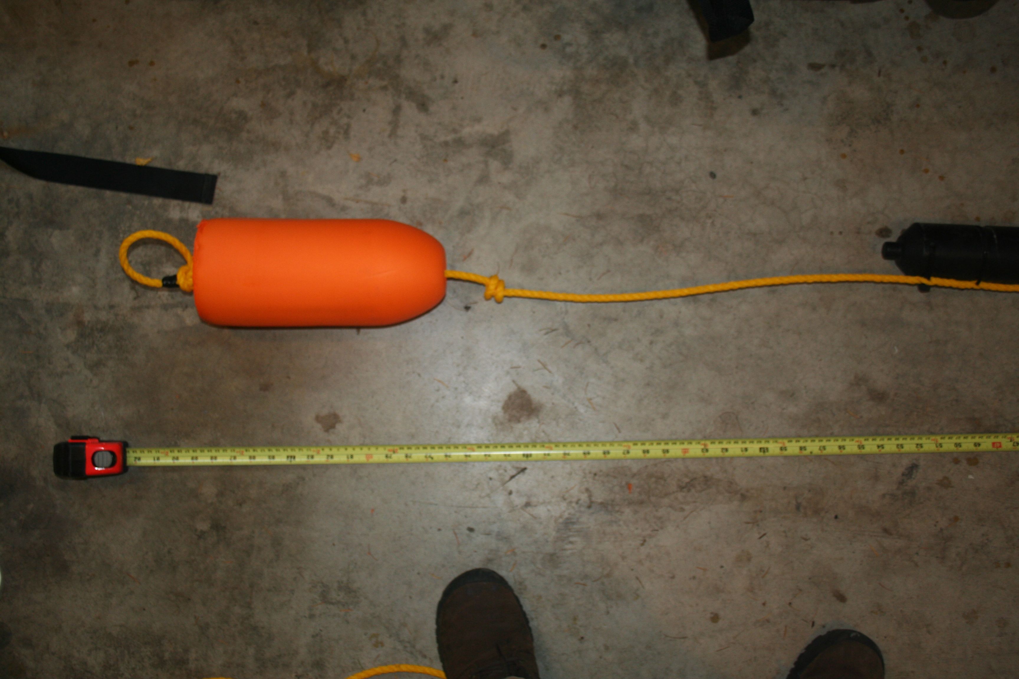
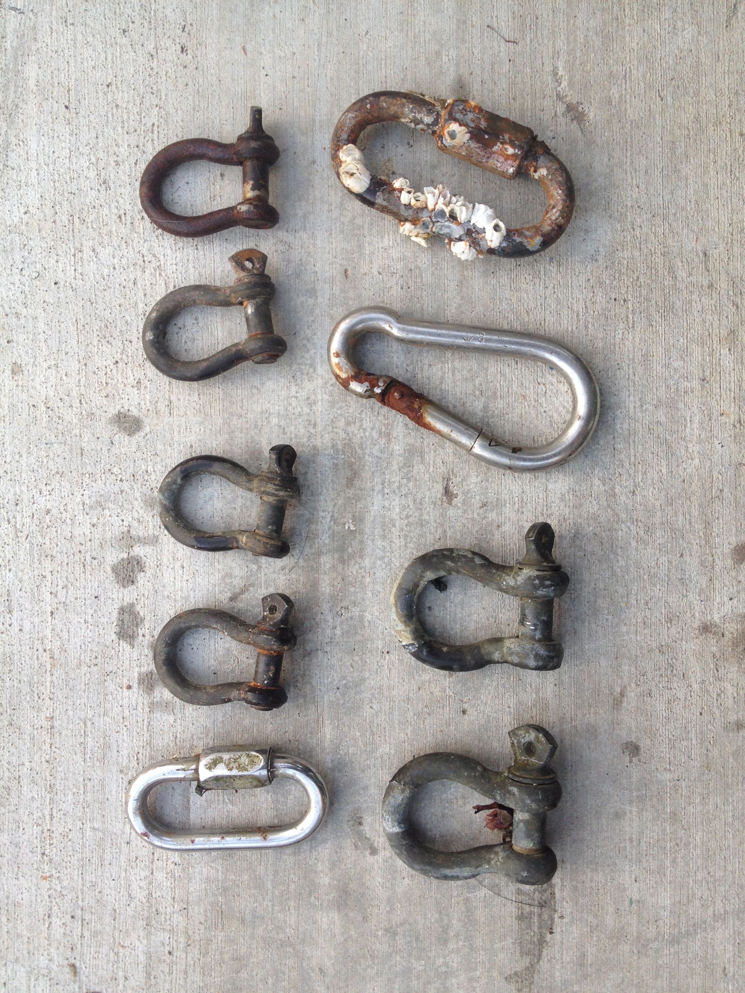
Tethered mooring materials, methods, and locations
Salmon school passes around the fish tag receiver mooring at Lime Kiln State Park
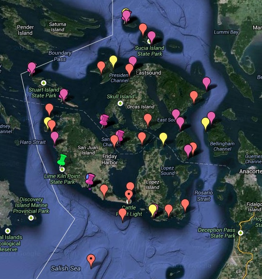
Project map (Google map in which green markers denote deployed receivers, magenta are recovered from our UW/NOAA collaboration (2011-2013), yellow were planned sites for 2011-12, red are other potential sites, and blue are landmarks):
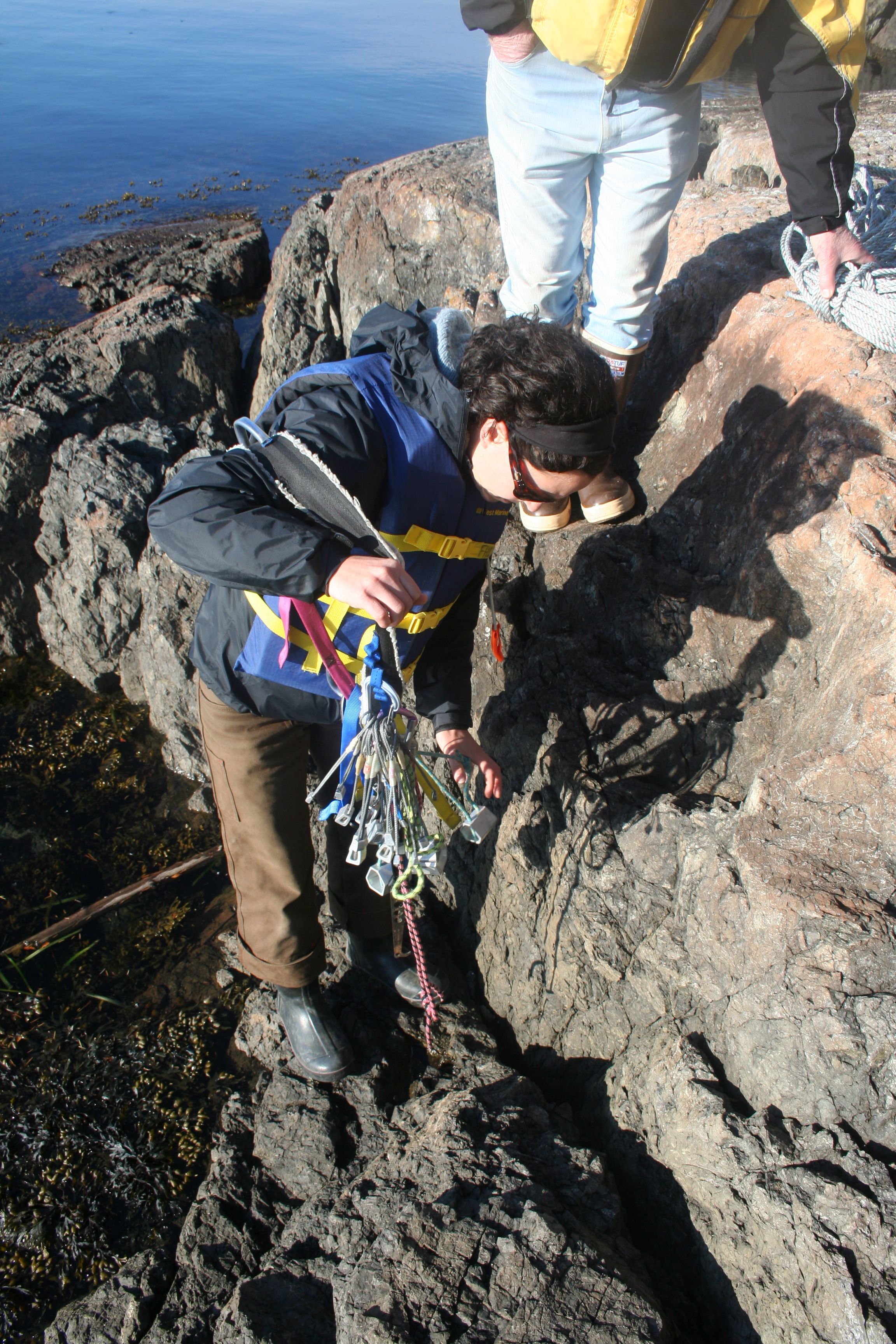
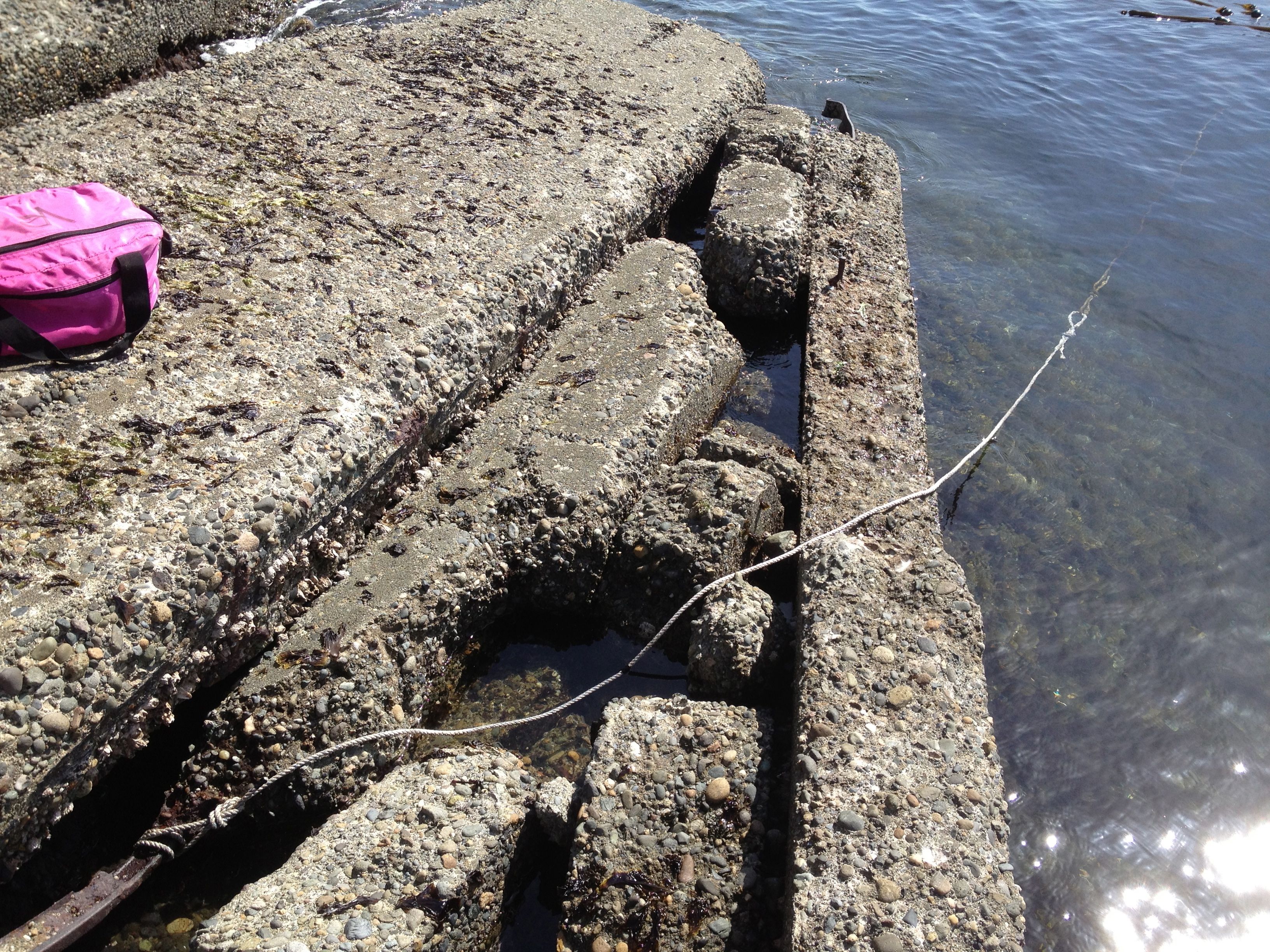
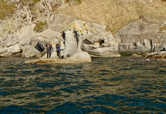
A typical deployment involved dropping a researcher off on shore. While the boat driver stood off and prepared the mooring, on shore the researcher created a climbing anchor using cracks of convenience in the rocks and/or trees. Aluminum alloy wired nuts, chocks, and hexes were the most common anchoring devices. Both seemed to weather the salt-water environment very well, though the stainless wire rope in the nuts and chocks showed some signs of corrosion after about a year in the field. Once set, the anchor was attached to a length of leaded crab pot line, a float was tied to the end, and the float was cast well offshore. The driver then returned to pick up the researcher and together they retrieved the float. The shore tether was then tied to the mooring and as the boat backed away from shore towards the deployment point, line and anchors were deployed until adequate water depth was attained. Finally, the mooring assembly was lowered into the water and released. (Early on we used a slip line, but eventually just dropped the moorings as they seemed to sink vertically and not too fast.)
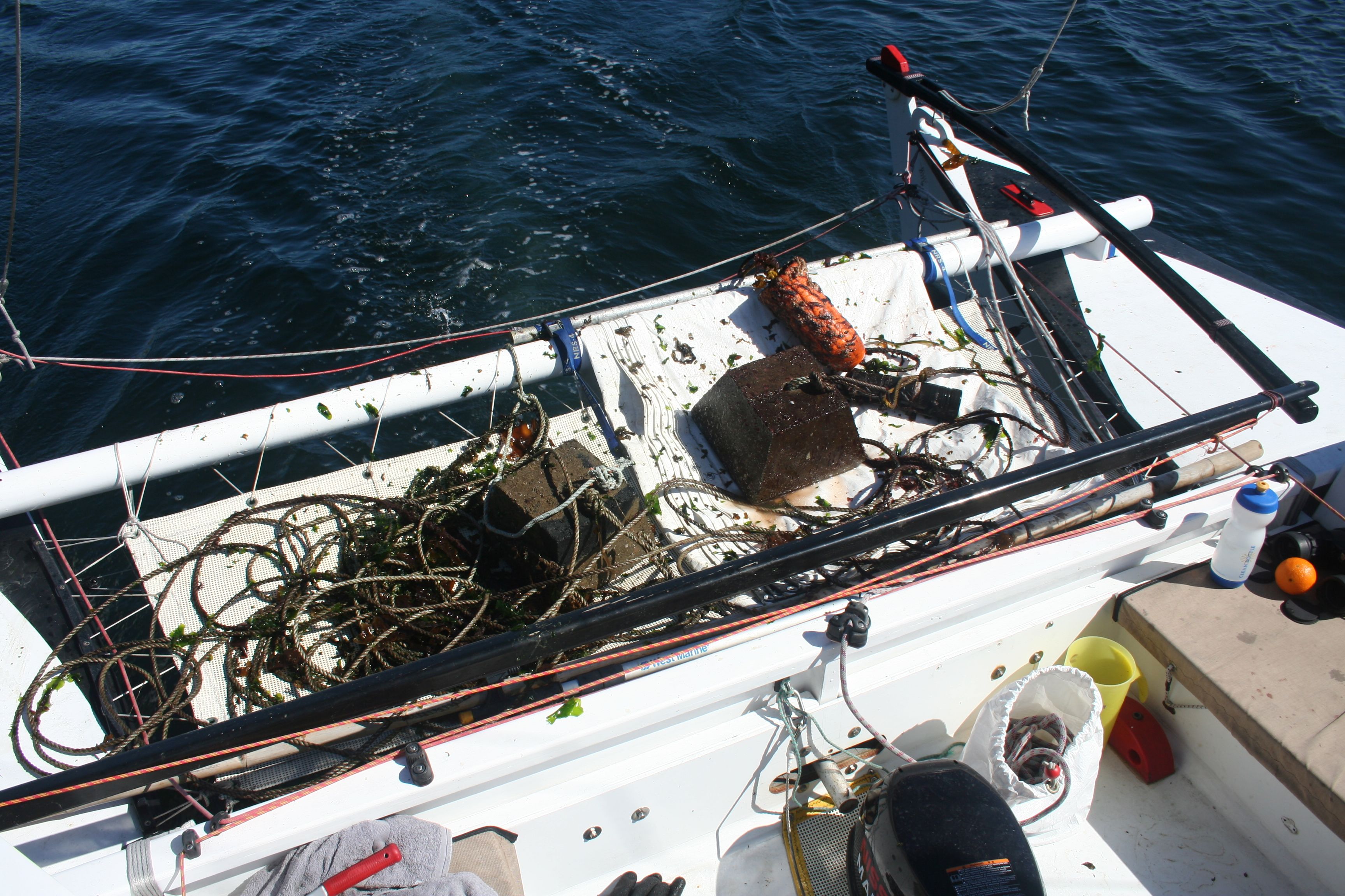
Recovery method
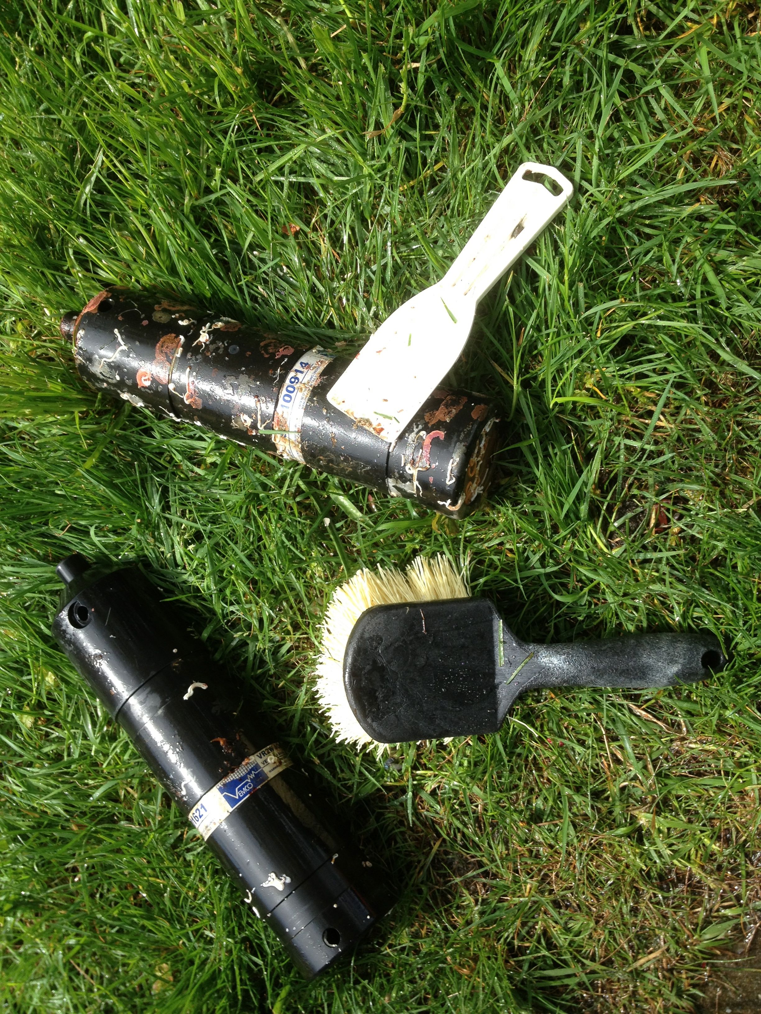
A typical recovery also began by dropping a researcher on shore. First the anchor was removed or checked and maintained. Then the tether was disconnected from the anchor and attached to a float. The float was cast offshore, the researcher picked up, and the float brought onboard. Then the dirty work of hauling up the mooring began. A bow roller helped, as did having two people work together. An important innovation was a short piece of PVC slit so that it could be passed around the line and used to strip fouling off as the line was brought aboard. Once the mooring was raised, the receiver could be removed or swapped. Then the mooring assembly could be stored or immediately reused in a new deployment.
With a small boat capable of doing 25 knots on flat water, this method allowed us to service 4-6 receivers per day. At the end of the study, we were able to retrieve 8 receivers in a single day trip beginning and ending in Seattle.
Lessons learned
Galvanic corrosion (between a stainless steel shackle and a length of galvanized chain) caused the loss of Lime Kiln receiver (luckily it was found on a beach near Victoria). Connect the Vemco to the mooring anchor using a single type of metal (e.g. a galvanized shackle).
Mooring depths should be at least 5-8 meters deep especially in high surge environments. Shallow deployments resulted in the loss of 2 False Bay receivers (one was found on a nearby beach).
Dive recoveries were required 4 times, primarily because of chafe (Iceberg, Sucia, Sentinel, Patos). Minimize tension and contact with rock edges?
Human disturbance rare (despite faded labels, only Turn Point and Obstruction were disturbed; neither was removed).
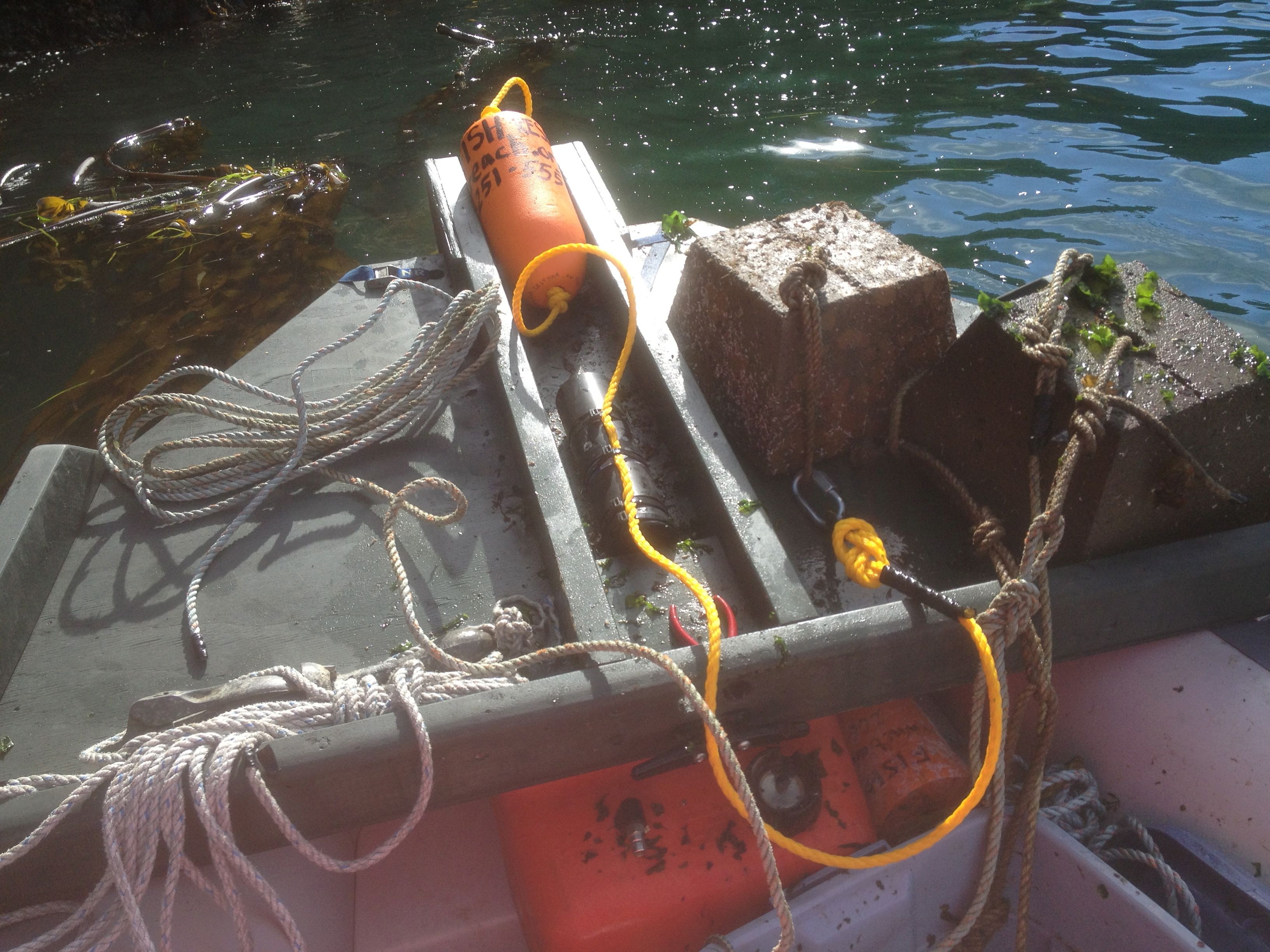
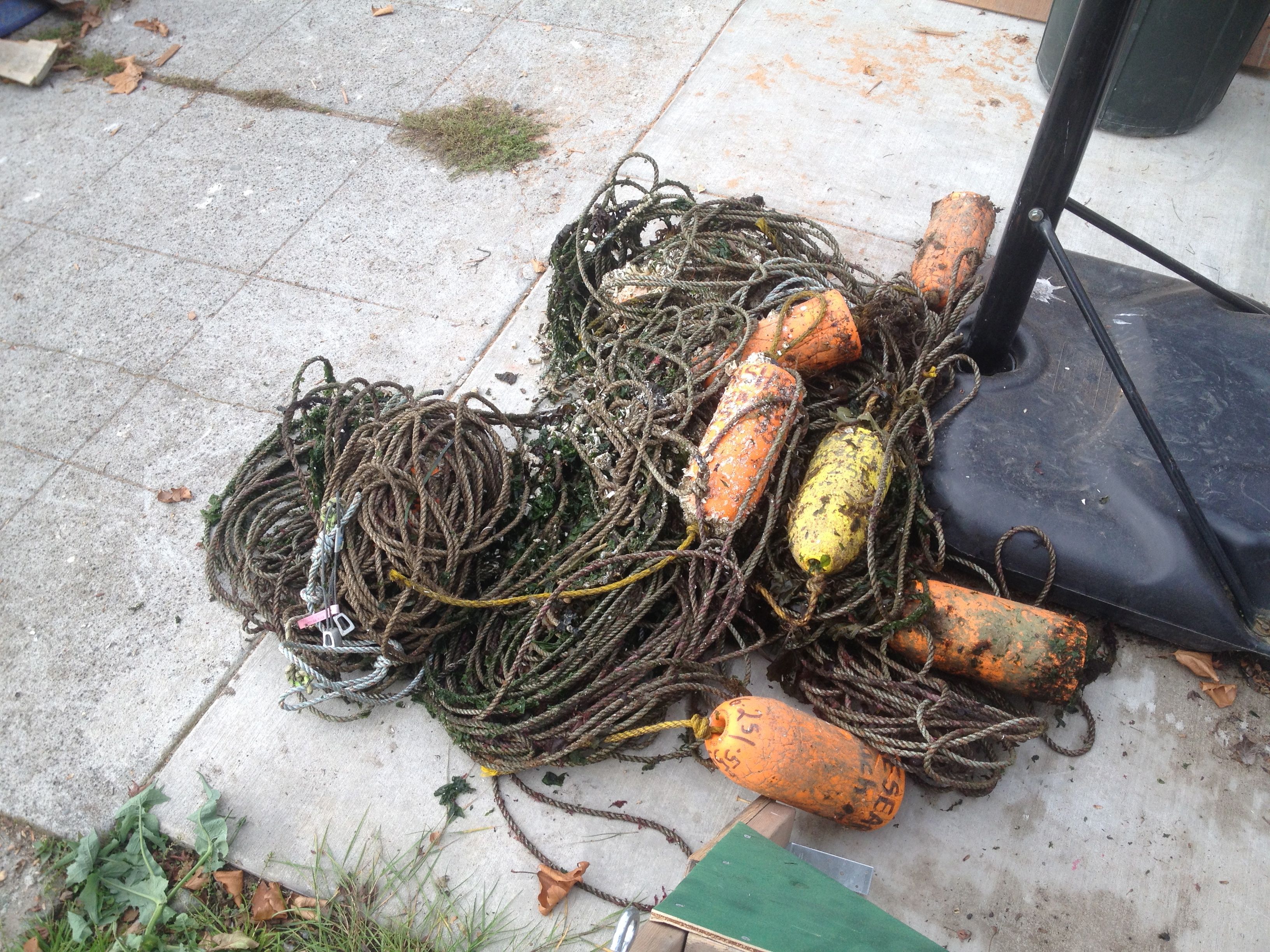
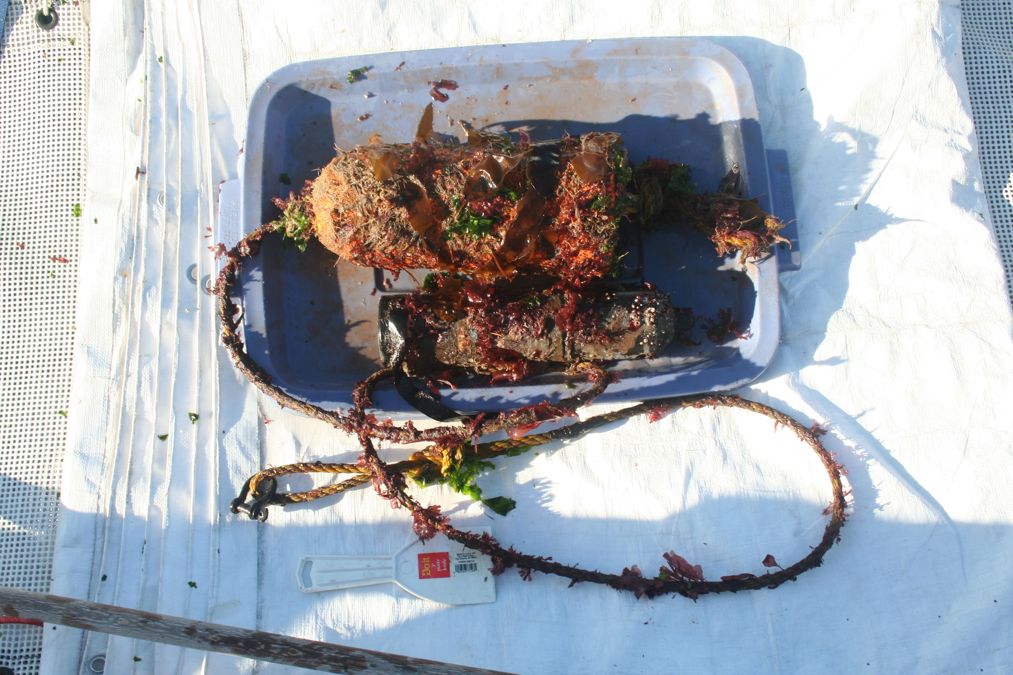
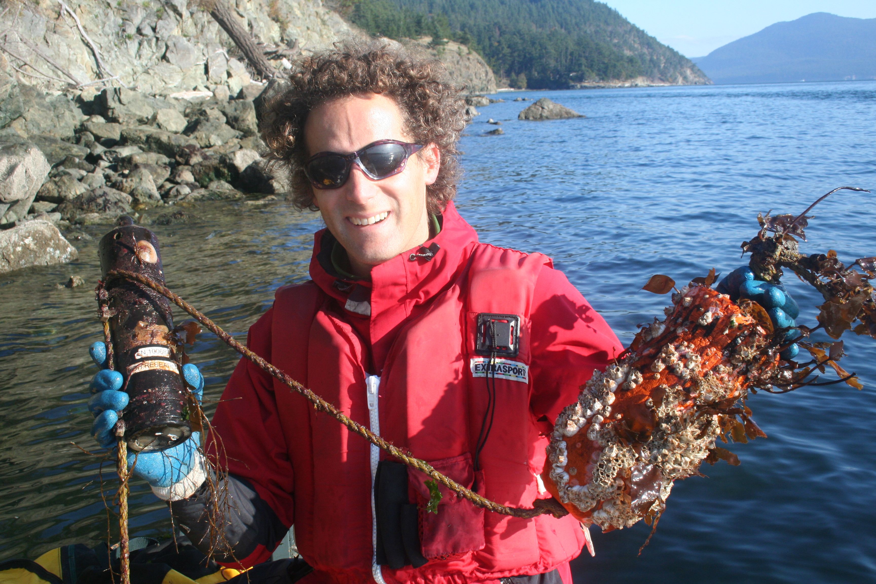
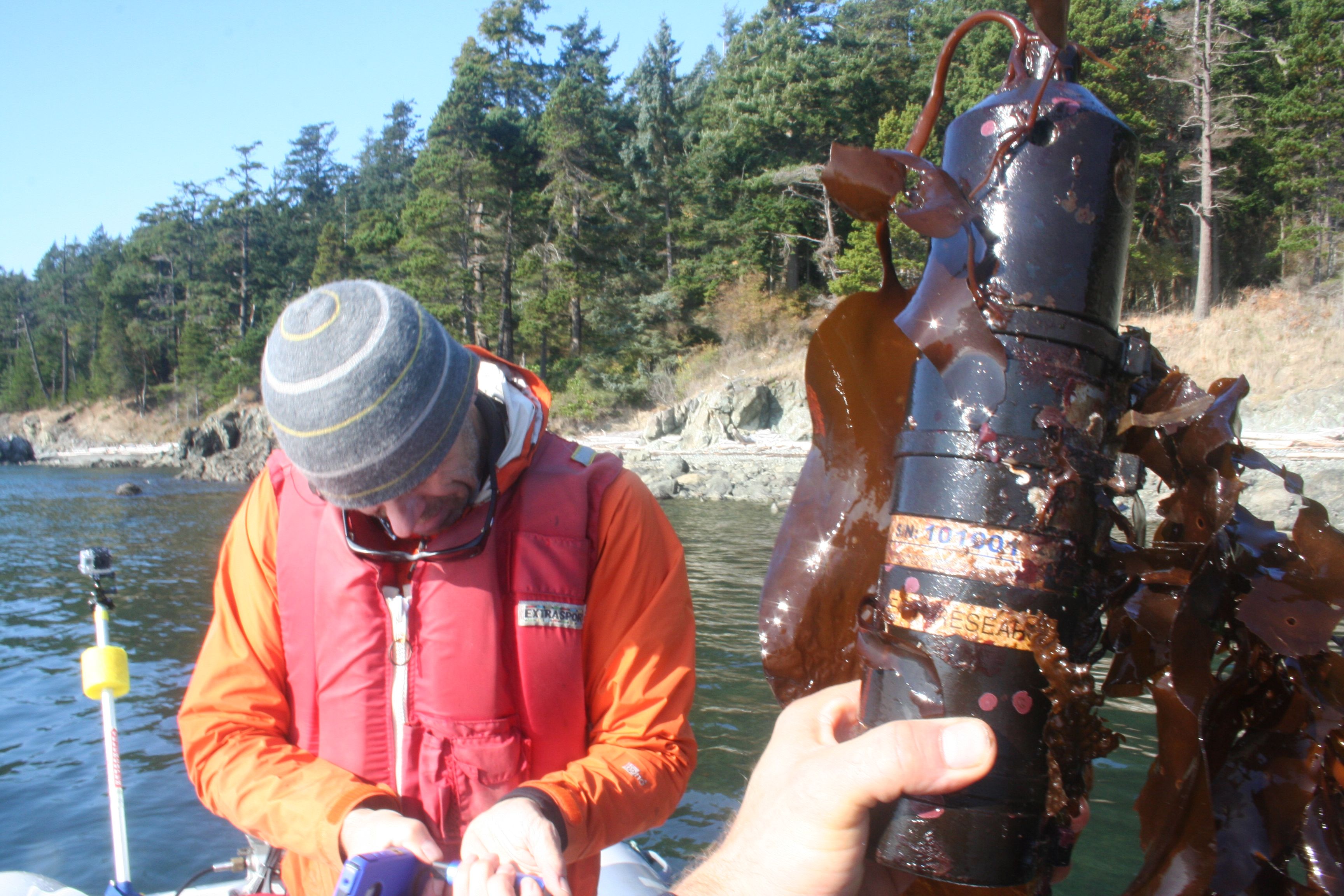
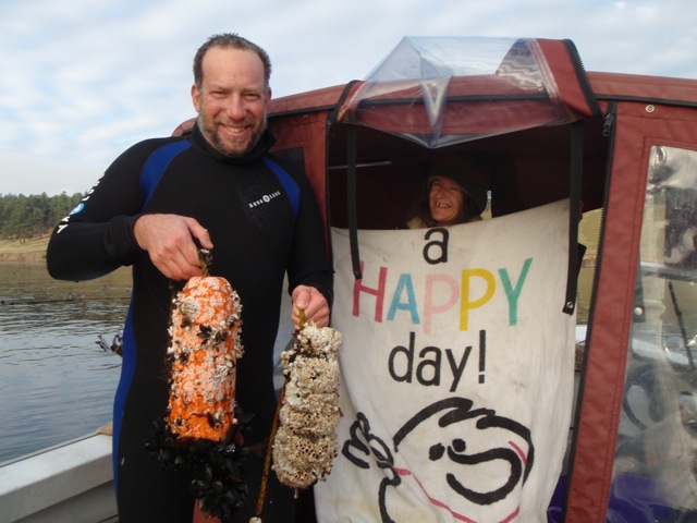
Examples of different amounts of fouling
The amount of marine organisms that colonize the mooring float, receiver, and/or anchor — as well as the line — varied tremendously between sites. Geography and oceanography are likely the controlling factors, but there was some suggestion that deeper deployments had less growth overall, and especially reduced amounts of brown algae colonization.
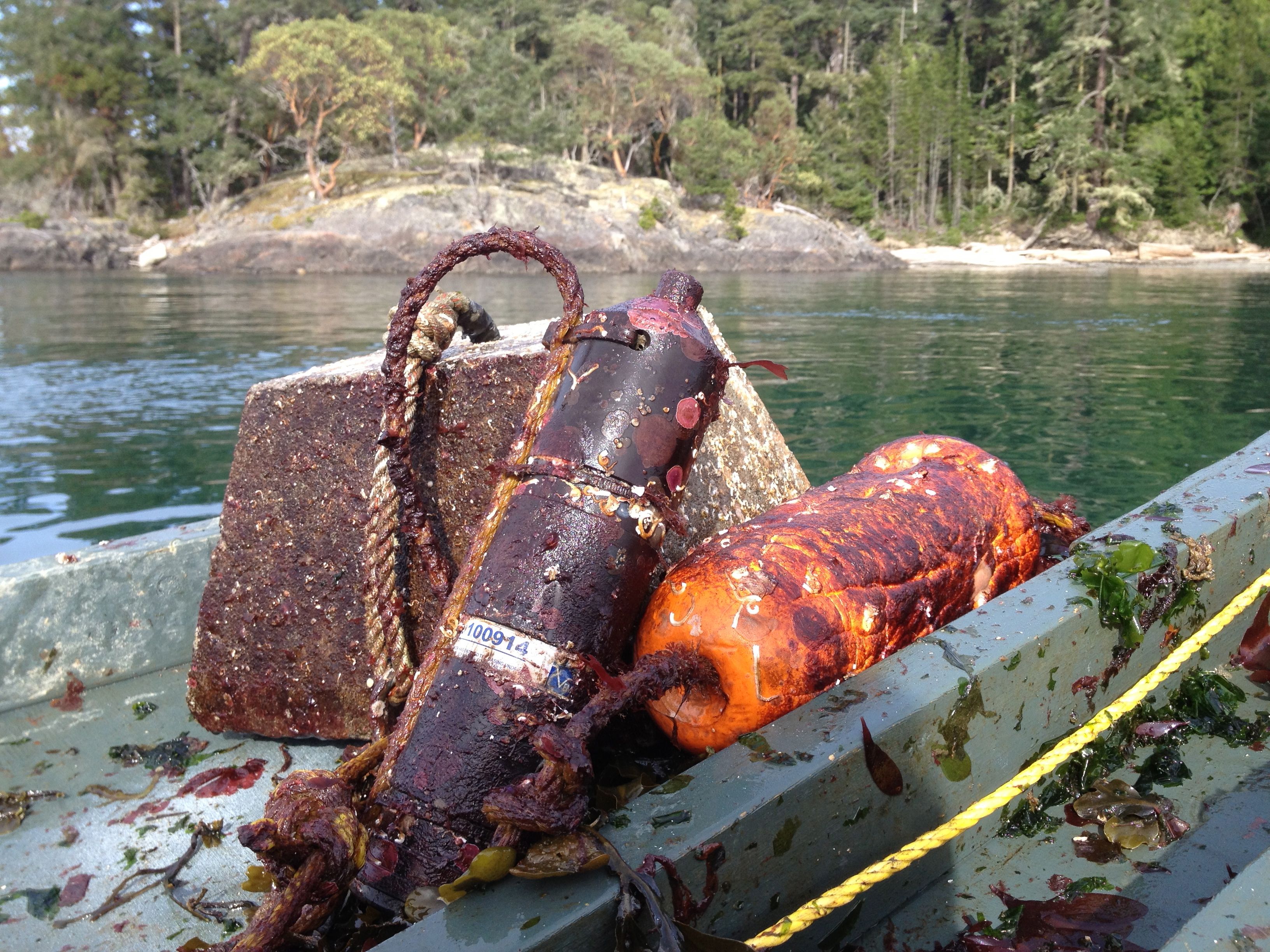
Sentinel 15 months @17m
Pt. George 17.5 months @13m
Undergraduate involvement
Unlike diving, this method allows students to assist in deployments and recoveries without specialized training. The method helps motivate new knot tying skills as well as small boat operations.
While Beam Reach students have not yet utilized data from the San Juan salmon tracking study, we hope that the Hydra database will facilitate that. To date, our only student projects using Vemco data came from our own tagging of ling cod at Lime Kiln State Park with pressure-sensing tags and monitoring achieved with a VR100 system.
Yesterday David Howitt and his crack team completed the retrieval of the last couple Vemco receivers that were being used to track adult salmon in our collaborative fish research with UW and NOAA/NWFSC. Here is David’s field report, along with some great photos:
Boat operator and two divers depart from Roche 1100, return Roche 15:30 – 4 1/2 hours
2 Dives, 2 retrievals, pretty straight forward with finding near shore anchor block early in dive at Succia. Sentinel found drifting line, went down to 60 feet and were lucky
Will deliver pier blocks, Vemcos and tanks to Val tomorrow
found one weight belt at Succia, lost one knife.
Succia Vermco SN# 100913
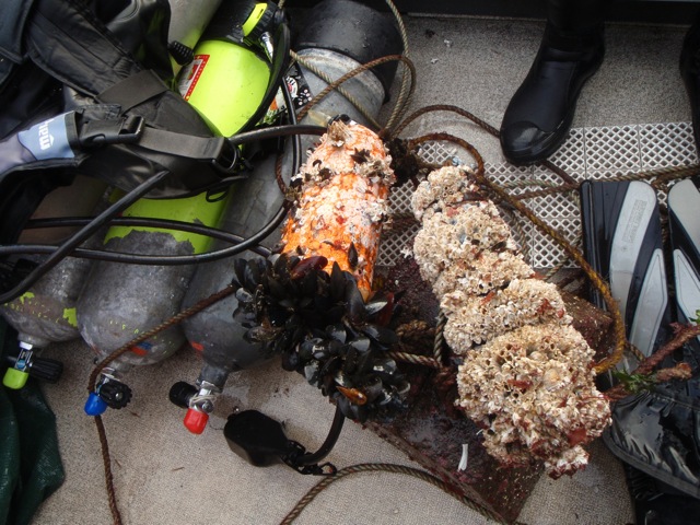
Sentinel Vemco barnacle encrusted
Pouring hot tea into gloves really helped
Dive stats:
#1 Sucia, 11:57 minutes,   41.56’,      46 degrees in water.
#2 Sentinel, 12 minutes,      62.25’,      45 degrees in water.
Note the water temperature! Bravo to David and his tough team for finishing the field work in the depths of winter!!
Divers atop the rock outcrop which served as shore anchor for the Sucia receiver.
Encrusted receiver and float atop dive tanks
Map showing all the receivers retrieved (in magenta) at the end of our San Juan Island salmon tracking study. Only one receiver remains — at Lime Kiln.
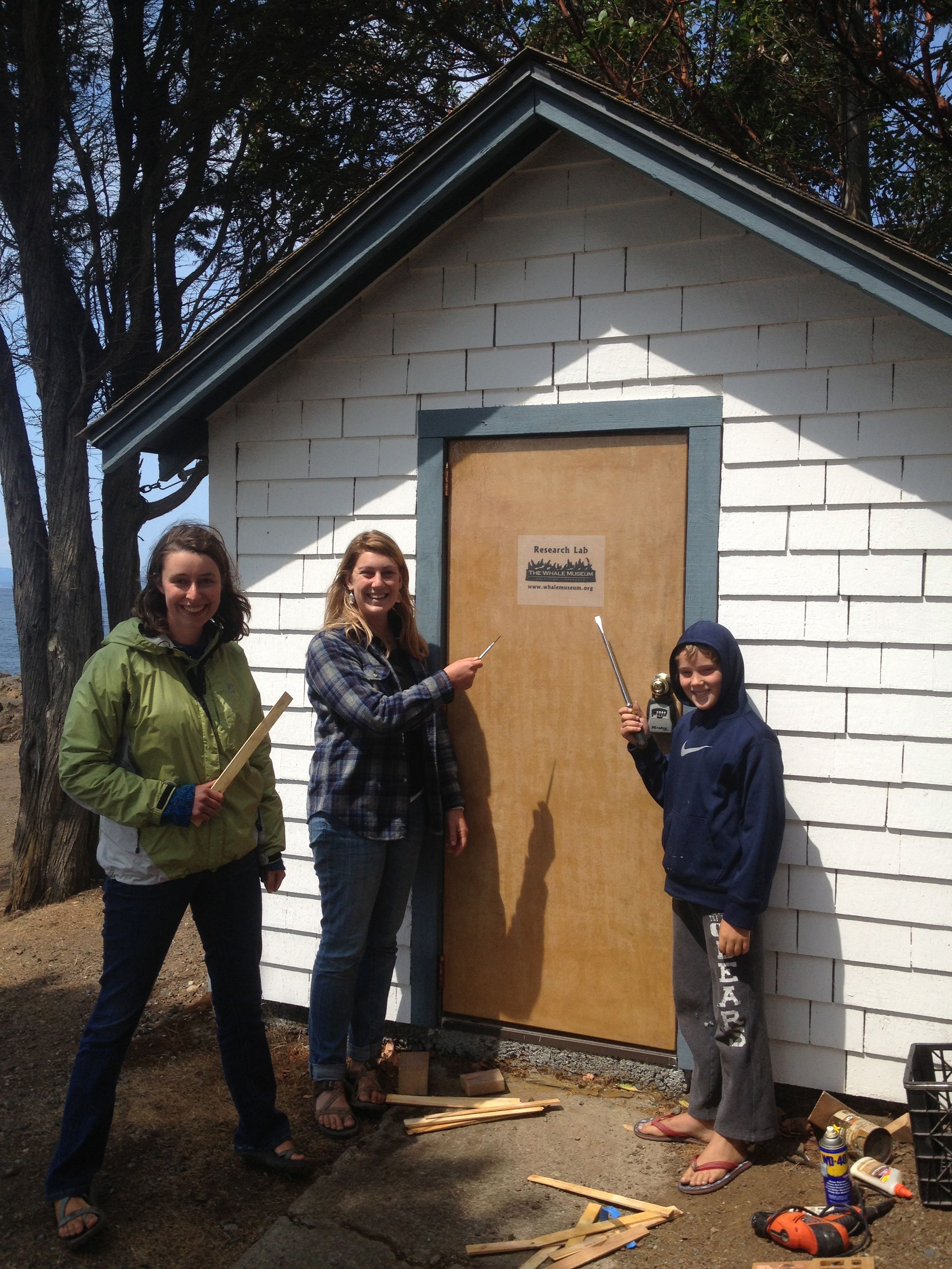
Today the Whale Museum Research Curator Eric Eisenhardt and his son Given helped install a new door on the acoustics shed adjacent to the Lime Kiln lighthouse. While the Beam Reach students had given the shed a face lift a few years ago (de-mossed roof, new paint, better drainage), the old door had been looking severely abused by the southerly storms and sun for a long time. The Whale Museum procured a new door about a year ago and I agreed to fiberglass it so it could better stand up to the elements and Neptune’s wrath.
After measuring and planning a bit with Eric, Liam, Bre, and Carrie lent hands with a absolutely STUNNING outcome: the door fit perfectly on the very first try! Normally, I gather there is some back and forth on mortice depth, planing the frame, or adjusting strike plates, but it all just worked. We screwed in two screws and the door swung right into its frame. We swung it out and put in the rest of the screws, and it still swung into the frame with only a gentle push from the wind. Then we put the handle back on and it swung in and clicked shut. STUNNING.
Anyways, it will need some paint (and a little polyurethane to protect the door label Jenny designed), but the door is in place! A special thanks to Bre for volunteering to dispose of the door in a ceremonial fire at her place.
Today (3/7/2013) marks the anniversary of the cranial dissection of L-112, a 3-year-old southern resident killer whale that was found dead at Long Beach on February 11, 2012. More than a year after her death, we are still gathering information about her case and many questions remain unanswered. Acoustic recordings made on the outer coast that winter are undergoing or await analysis and publication, final details from the initial and cranial necropsies have not been fully reported, and CT scans and dissection of the middle/inner ear bones are pending. There is not yet scientific consensus regarding key questions, including “What was the cause of her trauma?” and “Approximately how long was she dead before being discovered on the beach?”
In pursuit of answers and as a contribution to gathering all relevant data, today we present the edited footage from the cranial dissection of L-112/Victoria/Sooke and offer the raw footage to interested parties. Below is a 1-hour-long (1:09:03) distillation of almost 5 hours of raw footage from two Flip HD cameras. This is a synopsis of the dissection, including all audible commentary regarding trauma observations made by members of the necropsy team.
The synopsis is mostly chronological, but some effort has been made to group footage anatomically, with an emphasis on sound production and reception. There are titled sections on the following topics:
0:00:16 Disclaimer and introduction
0:05:57 Sampling blubber and skin (for Ted Cranford)
0:07:29 Removal of skin and blubber
0:13:30 Examination of the blow hole
0:14:24 Dissection of the melon
0:16:56 Phonic lips (with insights from Jason Wood)
0:49:17 Dissection of auditory bullae (bony structures containing middle and inner ear)
0:57:49 Upper jaw teeth (12 on each side!)
1:01:04 Narration: transition from bullae to brain
1:01:55 Discussion of inner ears
1:04:35 Removal of the brain
We have not included the archived footage from live-streaming of the necropsy, nor have we incorporated the many still photographs that were taken by Beam Reach staff, Sandy Buckley the necropsy team photographer, or others who documented the dissection. We welcome further efforts to assimilate all available information and in that spirit have included the above video and all raw footage collected by Beam Reach in our web-site-wide creative commons license (non-commercial attributed derivative works are permitted).
Later this spring in partnership with zoologist Dr. Kevin Flick of Poke the Dead Thing we plan to release a shorter (~20 minute) version of this footage for interested 6-12th-grade educators and marine naturalists. Key anatomical footage will be supplemented with diagrams, animations, and descriptions of bioacoustic functionality from the recent primary literature. In the interim, students and educators may enjoy studying the DOSITS overview of cetaceans’ fully aquatic ear and marine mammal sound production.
Another Vemco fish tag receiver was replaced today, helping prepare for another season of tracking blackmouth (resident Chinook salmon) in the San Juan Islands. This wintertime field work is part of a collaboration between Beam Reach, Tom Quinn’s lab at the University of Washington, and Kurt Fresh and Anna Kagley of NOAA’s Northwest Fisheries Science Center. You can follow our efforts at http://www.beamreach.org/fish-research
David Howitt and I dove from Val’s and Leslie’s shoreline (Orcasound, about 5 km north of Lime Kiln) into a sunlit, calm, and clear Haro Strait in search of a tether which was torn from its shore anchor last year. Luckily we found a frayed knot of the old line still attached to a sub-tidal boulder. Trailing a new tether (0.5 cm crab pot line) fed to us from shore by Ali and Val, we were able to follow the old tether out about 30 m to find a Vemco receiver (#100463) still attached to its concrete anchor at a depth of 8 m.
Old Vemco
New Vemco
Interestingly, the concrete block (a 25 kg custom-cast 30 cm square about 15 cm thick) had been flipped over. This could have happened when the lowering line was slipped last spring, or perhaps the currents tipped it over. Also, the stainless steel snap shackle was still attached to a stainless steel U-bolt that was cemented into the block, but there was clear evidence of galvanic corrosion. Future moorings should avoid such metal-metal contact, even for similar noble metals like slightly different types of stainless steel. The best way we’ve to avoid corrosion but make swapping receiver-float assemblies is to drill through a pier block and then thread crab pot line up through it to provide an attachment loop for a snap/shackle.
We removed the old VR2W and replaced it with a new one (#101594), being sure to back up the corroded loop with the end of the crab pot line. Then we swam back to shore and secured the crab pot line to a shore anchor (piton in an old bolt hole).
New shore anchor (with hydrophone pipe in background)
Unfortunately, no data was immediately available from the recovered VR2W because the receiver’s bluetooth chip has failed. The battery was discharged to such an extent during the deployment that the receiver went into what Matt at Vemco described as a “brown-out mode.” This apparently is known to corrupt the bluetooth chip on the receiver motherboard and requires returning the receiver to Vemco for a new board (~$250 Canadian). So, we’ll have to await repairs before we know whether any fish were detected at Orcasound in the last year or so.
Last June (2012) marine mammal researchers and stewards around the Pacific Northwest were surprised to learn of seismic research cruises that would use air guns to survey faults and crustal structure on the outer coast of Washington and Oregon. Our concern was that there would be inadequate mitigation of potential acoustic impacts on marine species (particularly southern resident killer whales). It all happened very fast and I never heard much about how it went… until now.
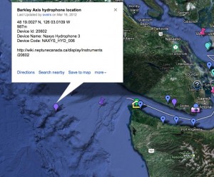
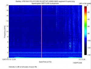
Thanks to John Dorocicz who has been logging acoustic highlights from one of the hydrophones maintained by NEPTUNE Canada near the head of Barkley Canyon, I just had the rare opportunity of hearing airgun blasts in the real ocean — complete with simultaneous vocalization of nearby dolphins. The date and time of the recording match up very well with a cruise track of the R/V Langseth, the research vessel from Columbia University’s Lamont Doherty Earth Observatory.
Here’s where the Barkley Canyon hydrophone is located:
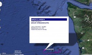
Here’s where marinetraffic.com AIS shows the Langseth was at 8:25 UTC on 2012-07-19, about 175 km south of the hydrophone.
And finally, here is a spectrogram of two seismic blasts recorded at 10:13 on the same day, along with sounds from (likely Pacific White-sided?) dolphins.
Listen to the recording and you’ll notice the low-frequency rumbles of the airgun blasts along with what seems like an increase in dolphin vocalizations (visible as wiggles at 4-6 kHz in the last fifth of the spectrogram). I wonder if these were the first two blasts the dolphins experienced. If so, then the suggestion (made by John initially) that the dolphins are responding to the blasts seems tenable. But were there many blasts before this recording was made? And why wouldn’t they react as much to the first blast in this recording as they seem to react to the second blast?
Regardless of the answers, it is exciting to hear what airguns sound like on Washington’s outer coast at a range of nearly 200 km. The number of marine animals exposed to the sounds of seismic exploration is staggering and begs the question: is the risk of interfering with so many oceanic lives worth knowing more about the subduction zone that may someday rock our west coast cities?
Exciting aspects of the workshop III agenda are presentations by Mike Ford on diet and distribution of SRKWs, Sandie O’Neill on contaminant and stable isotope insights, Sam Wasser on hormone analyses, John Durban on growth and body condition, and Dawn Noren about energy requirements.
Most presentations (will) include links to the slides (PDF or PPT) archived on the workshop web site. Select presentations also include a link to the audio recording of the presentation.
Day 1 (Tuesday, 9/18/2012, 8am-5pm)
8:16 Pat of WA Dept of Fish and Wildlife comments (mp3)
Generally agree with draft report regarding the low impact of extant fisheries on killer whale recovery.
But, in sections 5.2 and 5.3 the report mentions the distribution of “far north-migrating” Chinook stocks. Coded wire tag and genetic data from off WA coast show that many stocks are present, including: Sacramento and Northern Oregon coast. Columbia river summer chinook do sometimes wander into the Strait of Juan de Fuca or the San Juans.
Need more data on winter distribution of SRKWs.
There maybe thresholds effects, but they may be hard to detect.
Eric Eisenhardt comments:
SRKWs did go north of Vancouver island twice this summer, so that confirms they are foraging outside of Puget Sound and the Northwest Straits
L-112 Victoria/Sooke had both Chinook salmon and halibut in her stomach.
8:36 John Carlisle of Alaska Department of Fish and Game comments (mp3)
Growth rate criteria may not be the best metric for recovery. The growth rate will ultimately decrease as the population reaches carrying capacity. If you go to an abundance-based criterion, you’d conclude that the population is going to recover. Since the aquaria removals this population has been recovering.
Comment from Ken Balcomb (cutting through the smoke and mirrors): if you choose any decade other than the mid-70s when the population was at its lowest, the SRKW population is in decline, not growing. There were 100-120 before the captures; there are 84 now. That’s a decline in my book.
Comment: we ought to look at where these animals in every month of the year.
Mamorek and Ford: we are not being consistent yet about defining each season.
9:01 John Ford of Northwest Fisheries Science Center comments (mp3)
Reminded audience of workshop I and II data showing movements along outer coast at least from January through July.
Diet information was under-emphasized. We had more than two samples and we have new data.
Report makes overly simple assumptions about seasonal distribution
There is seasonal overlap of whales and Chinook stocks (they don’t feed only in the Salish Sea during the summer).
We need to be very clear about seasons and could look at shorter-time-scale overlap.
Not all versions of Ward’s lambda are comparable with the recovery growth rate criterion.
Comment discussion (Bain, Durban, Ward) of whether the SRKW abundance time series shows density dependence or not.
9:22 Department of Fisheries and Oceans comments (mp3)
Status of SRKW
the panel inference of increase (rather than decline) is stronger than warranted given inherent uncertainties (ref Velez talk later this morning)
causation is evidenced by multiple lines, including CPUE declining with decreased Chinook abundance
Feeding habits
Winter ecology could benefit from synthesizing information from w0rkshops 1 & 2, including all new acoustic and visual observations.
Diet data for Dec-Apr are scarce, but Chinook still appear to be primary prey.
Statistical design of diet studies should be undertaken
Fisheries and prey availability
Vast majority of Chinook eaten May-September are Fraser Stocks, but only weak association between terminal run of Fraser Chinook and SRKW vital rates. Why? Low quality data on Fraser Chinook? Abundance of Fraser Chinook may be sufficient for current SRKW population size.
Scordino question: why isn’t satellite tagging being done in Canada? John Ford: we’re focusing on acoustic detections along outer coast to get better sense of timing during off-season periods.
Balcomb question: wrt statistical sampling — our scale and fecal samples are really only collectible during low sea states; those samples are/will-be difficult to obtain during the winter months offshore.
Marmorek question: Why isn’t there a stronger association between Fraser Chinook time series and vital rates? We’re not sure, but there is a strong correlation between coast-wide Chinook abundance and vital rates… Led to discussion of correlations… Mike Ford summarized by saying there’s no single stock that’s better than the coast-wide abundance index.
10:20 Antonio Velez-Espino — Killer Whale Demography (mp3)
Selected 1987-2011 demographic data [10 years less than Ward!], used 7 age/sex categories [different than Ward’s!), and defined lambda as the asymptotic population growth rate
SRKWs have greater vital rate variability, lower fecundity, and higher mortality, and higher proportion of post-reproductive females — compared with NRKWs.
SRKW are in mild decline of -0.91%, while NRKWs are in annual increase of 1.65% (which is below the current SRKW recovery criterion!)
48 individuals were captured or killed according to Olesiuk
Greatest effect on vital rates is due to young female survival
Maximum increase in pop growth is produced most by young and reproductive female fecundity.
Greatest increase to lambda (pop growth rate) comes from avoiding reductions to survival of young reproductive females and increasing their fecundity.
Comment: why did you start with 1987? Answer: this was a compromise between extent and highest quality data that is most representative of the current population ~25 years or one generation back.
11:00 Mike Ford Review of southern resident diet information by season (mp3)
Cloning and high-throughput sequencing (extract DNA from homogenized and pooled from about 1000 prey samples and 300 fecal samples from a period of years (Jan-Apr not well represented); use primers for potential prey, not SRKWs; use reference and custom data bases of 40,000 DNA sequences; post-processing to remove chimeras) which has potential sources of bias (from collecting to relative tissue density of mitochondria, digestion factors, PCR amplification differences)
Results: May-July dominated by chinook; Aug-Sept include some sockeye and coho; Oct-Dec mostly chum (~3x more chinook than chum in Oct and Dec, but ~2x chinook more than chum in November); 2005-2008 August was highest proportion (~15%) of sockeye (Chinook made up the rest); Most fish were year 2-4, but some younger during winter in Puget Sound.
Jan-Mar only a handful of samples, but almost entirely Chinook.
Is this a summary of Salish Sea only? Yes, all fecal samples for summer months are from inland waters, though there are some samples (from John) from the outer coast…
Q: John Ford — Have you looked at samples that may contain prey transported by SRKWs as they return from an excursion to the outer coast. A: no due to budget constraints we have combined samples to look at average patterns.
Mike Ford: We haven’t tried to quantify the levels of DNA in the fecal samples from L-112, but we have detected Chinook and halibut.
Ken: wrt oct-dec sampling, all three pods were in the area during that point
Tim from NOAA fisheries: 2010 was our world record sockeye year. Mike: we sadly have no samples from those months in that year. Tim: there are blackmouth present during chum runs.
These methods differ, but are complimentary (stable isotopes average longer spatial and temporal scales)
D. Herman studied stable isotopes of KWs and prey that provide TEFs that help interpret our mixing model which shows SRKW stable isotope signatures along the “salmon line” in a location that our “classic” model says is associated with a diet in late summer of 43% Chinook (scales suggest 70%; fecal suggest range…)
An “alternative” model gives more weight to known prey choices and lets us ask what would TEFs need to be for results to be consistent with scale and genetic data?
52 scales samples (NWFSC only) (2004-2008?)
Estimated diet with scales (no genetic prior) = 72% median Chinook proportion
Median nitrogen TEF 1.65; carbon 1.18 (lower than reported)
Main result from all models: Chinook is dominant in September, but proportion is a little lower than expected.
Time-frame represented by biopsy samples (from about 12 of about 30 available SRKW samples) were selected to be from period of Aug-Sep, but we don’t know over what time scale the sampled isotopes are influenced…
Hypotheses:
SRKW eat more juvenile Chinook than we think
SRKW eat some other lower trophic species that’s not detected well in prey and scale samples (possibilities: BC halibut is left of salmon line; lingcod, rockfish, herring, and English sole are all to right [higher deltaC%])
SRKW eating more chum, sockeye, or steelhead than are apparent in the scale samples
Isotope turnover rate is based on bottlenose dolphin skin growth rate of 72 days.
John Ford: 2 stranded SRKWs on outer coast showed stomach contents consistent with Chinook and squid. Have you looked at their stable isotope signature?
John Durban: might fasting affect isotope ratios in the skin biopsies? Dawn: mammals usually metabolize all fats before affecting proteins.
Daniel: trophic fractionation data may help with your mixing model (KWs are like most terrestrial predators ~3-5 for nitrogen)
Scordino question…
12:00 lunch break
13:21 Sandie O’Neill — Using chemical fingerprints in salmon and whales to infer prey (mp3)
Contaminants in fish (POPs = PCBs, PBDEs, hexachlorobenzenes (HCB), etc.)
How do west coast Chinook salmon populations differ in POP concentration (about 30 fish from each of Skeena, Fraser (S. Thompson, upper/middle Fraser; no Harrison yet), Columbia River, Sacramento/San-Juaquin; about 80 from Puget Sound)
Puget Sound PCB levels about 4x higher than other sites (~60 ppb and highly variable — 10-210 ppb, migratory-resident); sub-adult residents ~140 ppb mean…
Multi-dimensional scaling plot (4 POPs) show similarity of samples: groups show Skeena is more distinct from CA, than Fraser is distinct from Columbia, with distinct and bimodal Puget Sound Chinook. Herring show similar geographic grouping of this pelagic signal, but benthic species show more local non/urban-patterns.
K/L pod fingerprints overlap with CA/Columbia fish; J pod overlaps most with Puget Sound non-resident Chinook.
13:50 Michael Ford — Overlap of southern resident killer whales and Chinook salmon (mp3)
What we really want is overlap of SRKW and Chinook along west coast over time.
Figure from first workshop: Daily SRKW (all pods, and J pod alone) sightings 2003-9 is above 75% for May-July, above 40 in Aug-Oct.
K/L pods not showing up more than 50% of the time until June
Slide with inference of time spent in regions offshore of CA, OR, WA, BC by Ken B (too small to see values)
Acoustic recorders of Brad and John show SRKW (mostly K/L) detections per unit effort peaking at 10% during Jan-Mar at Columbia, but also significant during winter as far south as Point Reyes. Riera plot shows seasonal pattern of NRKW and SRKW at mouth of Strait of Juan de Fuca.
Summarizing whale distribution
July-Sept 56% of time inland; 44% in western straits and Vancouver Island
April-June — 70% outer coast (~19% of days accounted for with PAM/NOAA — 65% centered on Columbia, 30% near Tatoosh, 5% south of Columbia.
Oct-Dec 81% outer coast, 19
Jan-Mar 96% (missed north-south breakdown), 4%
Chinook distributions (Weitkamp, 2010, coded wire tag data; May 2010 genetic data from WDFW, NMFS, DFO not covered here much but consistent with CWT results)
Summer — 56% inland; 44% western straits (more than 100 tags annually from lots of stocks — central BC to CA, including Columbia)
Spring — 68% of time outer coast (65% off Columbia to Olympic coast; 30% western straits; one more…)
Winter — 75% outer coast (75% Columbia/WA) 4% puget sound [Only about 6000 tags over 40 years of CWT effort; compare with summer total of ~110,000]
Fall — 81% outer coast
Whales spend ~40% of time west of Strait of Juan de Fuca
April-Dec SRKWs overlap with all major stocks south of central BC
Jan-Mar very limited salmon data
Ken Warheight WDFW samples from Chinook ocean troll fisheries off WA coast show 2011 May-Aug show lots of Columbia stocks, and other (mostly Oregon)
WCSGSI Collaboration by Pete Lawson and Renee Bellinger show genetic data: similar stocks present off OR coast.
Furthest south J pod has been detected on acoustic recorders is Westport.
Comment from Dave _____: CWT data show salmon distribution where fishing occurs, not necessarily their natural distributions; same commenter said “Columbia stocks spend their entire life history in the range of the SRKW” (!). The north OR coastals come in June when SRKWs are mostly in inland waters. M.F.: One of my main points is that in June, and especially May, K/L pods are spending at least half their time on the outer coast.
14:22 Antonio Velez-Espino, DFO — Role of ocean and terminal run abundance of Chinook salmon on Resident Killer Whale population viability (mp3)
1: Main hypotheses (based on diet evidence)
1a. SRKW growth influenced mainly by terminal run size of Fraser Early, Fraser Late, and PS Chinook
1.b NRKW Northern BC, Central BC, WCVI…
2: Additional hypotheses (assuming Chinook remains important diet component year-round) relate to stock size, spatial overlap, and temporal overlap
2a. SRKW growth influenced mainly by terminal run size of abundant stocks
2a. SRKW growth influenced mainly by ocean (pre-terminal) abundance of ocean-type stocks with large contributions to ocean fisheries
…
Again using 1987-2011 RKW abundance and vital rates, Kope-Parken terminal run size, CTC Cohort ocean abundance, simple * mulitple linear regression models
Results:
Some support for 1a and 2a; interestingly, most interactions occur with female 2 fecundity (old reproductive females)
Interactions with Puget Sound ocean abundance and young & old reproductive females; and WCVI are most important. (Both are selected for fisheries scenarios)
We, too, were surprised that the Puget Sound ocean abundance seems to be more important to SRKW population growth than the Fraser river stocks. It may be that there are confounding factors (e.g. toxins) or it may be we don’t have enough data to resolve what may be weak signals.
Physiology is a bridge — dynamic changes can be captured by allostatic load; reproduction can be suppressed by physiology.
Having many factors influence a given hormone is a strength!
Endangered caribou example
SRKW results (4 years)
GCs increases with psychologial and nutritional stress
Thyroid T3 decreases with nutritional stress, but changes more slowly than GC
Hi Thyroid corellates with high birth rates and low death rates
The more Chinook at the Columbia (or Fraser) river, the higher the mean T3 level
We get 150 POP samples/year (compare with O’Neill’s 30 biopsy samples) showing, e.g. PCB/DDT ratio for K/L pods is always much lower than for J pod
Guide mitigation
If fish matters most, recovering fish should be top priority (maybe not fisheries, but Habitat!)
Timing of run may be key (delaying fishery may help)
Measuring physiological response over time could also indicate how things improve in response to mitigation
Few tools can offer that
During last workshop, L10 (L90?) was thought to be injured. We’ve already resolved that she was pregnant and aborted!
There is tremendous variability from year-to-year in Fraser (Albion, 2007-2011; 66k-242k). In a year when there are long delays in the Fraser peak (near Julian day 240), it may be devastating if
Andrew Trites comment regarding possibility that thyroid data could be interpreted differently (referenced their captive starvation experiments and some studies in wild).
Lance Barrett-Leonard comment: we historically have observed that RKWs arrive in a condition of relative nutritional stress — e.g. ketosis, more foraging earlier/ more social later.
Comment: upper Columbia river stocks (Bonneville) aren’t caught in any ocean fisheries; lower Columbia and Willamette stocks are more impacted by ocean fisheries.
15:24 Break
15:53 John Durban — Size and body condition of southern residents (mp3)
Review of last fall’s results along with new analysis
New analysis regarding two comments made by NWFSC that suggest there has been a misunderstanding:
photogrammetry of Durban et al 2009 has high error rates.
photogrammetry did not detect that L67 was near death.
We used boats of known length to quantify bias of ~7cm at altitude of 1000′
But when we’re measuring distance ratios (relative shape), e.g. length/width, within the same photograph, altitude does not matter. Width is harder to measure than body width due to waves at edges of body, so we used head width/length to gauge error rates; average coefficient of variance only 0.03. L67 was only 0.12 when average female was ~0.135.
Latest efforts are looking at whole body shape differences between whales
L67 jumps out as having “peanut head” and anomalously thin peduncle
J14 and J17 were measured when around 12 months pregnant and found the peak of their width came aft of their dorsal fins.
Pitman et al, Journal of Mammalogy 88 demonstrates with Antarctic KWs where we hope to go with SRKWs.
16:16 Dawn Noren — Energy Requirements and Salmon Consumption by Southern Resident Killer Whales in their Summer Range (mp3)
RKWs (both N and S) are larger than Icelandic KWs (from which captive KWs have been used to get estimated length at age from time series data)
Best estimates of asymptotic body length of SRKWs come from captive Islandic whales — Females 630 cm; males 700 cm — and are also consistent with the initial photogrammetry results of Durban (when corrected by 80% factor?)
There are some times when SRKWs are estimated to consume upwards of 50-60% of some runs
Conclusions:
Two approaches to determine SRKW DPERs yield similar results.
Two approaches (Williams vs Hanson) do differ slightly…
Ray Hilborn question: is there scientific consensus about an annual cycle in killer whale condition?
Durban confirms that later in the summer social behaviors that create better grouping for photogrammetry
Barrett-Leonard makes another supporting point…
Bain mentions that other patterns suggest early stress (travel speeds get higher, echolocation rates higher)
Wasser suggests that they seem to have had their most energetic feeding of the year in the early spring; he may have said “best body condition,” but meant most energetic feeding.
How do we make population inferences from studies of individual whales.
Sam: it depends on number of samples you’re getting.
Longer discussion with comments from Ken B., Fred F., Dawn N., Lance B-L. (behaviors like prey preference and inertia are important), John D. (we should indeed reflect more than we have on our inferential framework).
Another panel member suggests it may be fruitful to conduct a meta-analysis of other populations (e.g. for population significance of a female that has a 100% offspring mortality).
John Ford suggests comparisons with transients would be useful, but we lack the detailed census information and behavioral observations we have for residents.
John Durban mentions recent completion of study of a few *thousand* resident KWs from northern climes (often feeding on acker-mackerel(?)) leads him to think that SRKWs are indeed unusual residents.
Most overlap in human and orca (Hanson samples) are Hein Bank to Henry Island; orcas not catching (or Brad not sampling) as much as recreational fishers inside east San Juans or Rosario; no fishers reporting from Pt Roberts area where orca prey samples were obtained.
Lummi Chinook bycatch in their sockeye fishery report mostly Fraser Chinook in Pt. Roberts/Alden Bank area.
Chinook proportions are much lower in recreational catch than in orca samples, with greatest difference in July (all areas of San Juans ~10% Chinook)
Fork length vs age: mean length ~55 cm in age 2, 70 age 3, 80 age 4, 90 age 5 (legal limit ~52)
In each area the same age class are about the same across 3 main stock groups.
There appears to be a difference in
Comment Tim of NOAA: sockeye migratory corridor changes from Rosario to Haro from year to year. Do Fraser Chinook do the same? A: The main reason there are proportionally more PS fish caught in Rosario area is that there are many more PS fish there; there are, though, some Fraser fish are present there. Tim: Skagit fish mill in the Anacortes area.
8:47 Robert Kope, NOAA — Effects of fishing on availability of Chinook salmon to resident killer whales (mp3)
Harvest impacts make up more than 20% of the “Parken-Kope” indices
The indices don’t account for immature (age 3-4) fish not killed by fisheries.
On average, these immature fish account for more than half the total abundance in the ocean.
How appropriate is the 20%? Harvest impacts account for 33% of the aggregate PK index.
What matters to the killer whales is the local density where they’re foraging. Abundance may be sort of irrelevant to RKWs. Overall, 20% seems like “a reasonable ball-park number.”
Bain question re whether immature fish are important to SRKWs that seem to prefer largest fish?
Alison question: Should we be considering outside stocks more? A: The fall aggregate mostly consists of outside stocks.
Panel question: Can we clarify salt-water age versus fresh-water age 2-5 terminology? A: Most stocks except Fraser spring Chinook have ocean-type (vs stream-type) life history.
Another public comment re Upper Columbia River Chinook not being available in the ocean fishery.
Larry Rutter comment: we should be very disciplined about the nuance between harvest rate and exploitation rate. A: Within a small group of the Pacific Salmon Treaty, there is a distinction harvest rate is “a reduction in the number of fish that are available.”
9:14 Robert Kope, NOAA (again) — Assessment tools for evaluating effects of salmon fishery management on resident killer whales (mp3)
Fishery assessment tools — FRAM vs CTC — use similar algorithms and ~95% same data.
Exploitation Rate Analysis (ERA) uses coded wire tag recoveries by brood year, typically available a year out (e.g. 2012 ERA used CWT data through 2010)
ERA, GSI, and Parken-Kope are retrospective
CTC, FRAM are both retrospective and prospective
Mark-recapture is the “gold standard” for estimates of escapement numbers which are used as model inputs.
Panel question: I’m concerned that we have model predictions with CVs of 50%. Ward A: forecasting beyond ~5 years is difficult.
Panel question: Is KW predation changing the natural mortality rate in a way that the FRAM model doesn’t capture because it uses a fixed natural mortality rate?
9:42 Antonio Velez-Espino — Chum salmon as a covariate of Resident Killer Whale population viability (mp3 | video)
Using BC and WA terminal runs of chum
Highest elasticity was for interaction between Puget Sound salmon stock aggregate and fecundity of young and mature reproductive females
10:40 Eric Ward — Estimating “other†marine mammal effects on salmon with limited data (mp3 | video)
How much to seals and sea lions compete with SRKWs?
Best U.S. data: harbor seal surveys (Jeffries et al., 2003); Canadian and other data sources have data gaps…
Panel suggested using Ecopath modeling results, but Eric has no confidence in model outputs.
Instead cite A. Acevedo-Gutierrez work or citations in his papers.
Better approach: multivariate state-space modeling using MARRS R package (Holmes+ 2012)
Essington & Quinn have survey data going back to 1930s/1940s, but data are messy.
Harbor seals are eating more juvenile Chinook than adults.
10:56 Scott Pearson, WDFW — Competition from Pinnipeds (mp3 | video)
3 pinnipeds overlap in range (but not necessarily time and niche)
Harbor seals: reaching carrying capacity in ~1990s (Jeffries, 2003)
California sea lions: all males in pulses from southern colonies
Stellar seal lions: population growing and continuing to grow in SRKW habitat
It’s complicated!
11:17 Lynne Barre & Eric Ward — Summary of lambda & Killer Whale growth rates (mp3 | video)
Delisting criteria: mean growth rate of 2.3% per year for 28 years
Info about population structure and behavior that is consistent with resilient (e.g. shorter inter-birth intervals)
Data supporting criteria
1974-1980 mean 2.6%
1984-1996 mean 2.3%
NRKW 1974-1991 3.4%…
Some have suggested abundance criteria instead of growth rate…
If you achieved growth rate of 2.3% from 81 whales in 2001, you’d get to 155 whales in 28 years (in 2029) => delisting
for 14 years you’d get 113 whales in 2015 => downlisting
11:23 Ward swaps with Barre, summarizes past lambda results, and presents discussion questions (starting ~11:30)
Mike Ford Q: extinction risk was influenced most by catastrophic events, so maybe an alternative de-listing criterion could be a threat criterion. Lynn A: we have quite a few threat criteria already.
Panel comment: Given the uncertainty in the historic population size, let’s say you used 1/2 carrying capacity. The estimates I have would put abundance at high 90s or even as high as 300. Ward A: one solution would be to optimize carrying capacity and growth rate. (balance productivity and abundance). In fisheries those are Kobe plots — exploitation rate and abundance are axes…
Larry comment: Back in Poet’s Cove, we asked “what’s the best think we could do for southern residents.” The answer was take care of Fraser salmon. Now it should be take care of Chinook salmon. Lynne response: one of our three components to the recovery plan is recovery of the prey populations.
Bain comment: An alternative is a recovery budget that starts with trying to conserve genetic diversity. At 3% growth, you lose 6% genetic diversity per generation. If you stay stable, you lose 25%. If you decline as in 1990s, you lose 50%. I’d like to see actions that try to achieve that 3% growth as soon as possible (WW impact reduction is fast but has short effect; toxin reduction is slow but has long effect; salmon recovery actions have a wide range that could be pieced together to get optimum evolution of population growth). Lynne A: there is a table in the recovery plan that is a basic approach similar to what you’ve mentioned. Dave: Incorporate a time frame into that.
Scordino Q: if you met your recovery goal and got up to 155 and then did your PVA would you still call it an endangered species? Lynne: I don’t know.
Scordino Q: if population stabilized and we determined the carrying capacity had been reached, would the SRKWs be delisted? Lynne: I can’t answer that now.
Mike Ford: We should tie recovery to risk of extinction, not carrying capacity metrics.
13:23 Eric Ward — Other approaches to adjusting Chinook abundance (mp3 | video)
Scenarios involving raising P-K index by 10%…
Why not other P-K indices? Best predictor is total index (aggregate of all salmon stocks), implies that no one stock is important in all years
13:36 Antonio Velez-Espino, DFO — Resident Killer Whales population viability analysis under selected fishing scenarios (mp3 | video)
4 scenarios
Under status quo, the ime for quasi-extinction of SRKW (population falling below 30) at median probability is ~50 years.
Under all scenarios, the probability of downlisting is always zero under U.S. criteria.
Only under most extreme (fishing reduction) scenario does the SRKW growth rate become positive!
Hypothesis 2a: closing WCVI fishing only increases growth rate by ~0.5%
75% reduction in ocean harvest rates of Puget Sound stocks also only results in ~0.5% growth increase
Is Chinook abundance limiting population growth and viability of RKW?
We need more research to understand depressed SRKW calf survival (relative to NRKW)…
First report will be available in February.
Panel comment: This seems opposite of what Eric Ward found. You’re saying they’re going to go extinct. A: Yes, unless dramatic change is made in fishing impacts, based on this time period we have chosen in which population is in decline.
Peter Olesiuk’s census data is of high quality for individuals during the period we chose.
Lots of discussion, primarily around why these results are different from Eric Ward’s.
14:23 Panel presentations about causality vs correlation (mp3 | video)
 5 panel members:
Jim Irvine
Dave Bernard, ADFG
John Ford, DFO
Scott Pearson, WDFW
Eric Ward, NOAA
 Panelist 2: CA fish have been notable in their rarely being mentioned in these workshops. We have a correlation between lower Columbia stocks. I find it ironic that we aren’t looking at the stocks that seem to be important to the SRKWs.
John Ford: 1990 decline of SRKWs coincident with prolonged decline in coast-wide salmon stocks is revealing. Mortality indices during late 1990s were 3-5 times higher — unprecedented. SRKWs are resilient to 1-2 years of nutritional stress, but not more. 8 of 13 peanut head cases occurred during years of low Chinook abundance.
Scott Pearson: Chinook are clearly important in both summer inland and winter outer coast habitats. You could look at evidence ratios, but Eric provides reasonable cut-offs that show that Chinook are important. The relationship makes biological sense, but seems to not have a strong effect on SRKW population dynamics. We’re dealing with a species with vital rates that don’t respond quickly. We extremely good data on the killer whales in contrast with fish data that have high coefficients of variation.
Eric Ward: The N & S RKWs population dynamics are correlated which suggests a bottom-up trophic effect is main control. This is a predator-prey issue in which we know very little about their winter diet, especially historically. So, I’m confident it is a salmon story, but maybe not a 100% Chinook story.
14:52 10-minute coffee break15:10 Panel presentations about effect of fisheries (mp3Â | video)
Eric Ward: Pinnipeds seem to matter, e.g. SJI harbor seals consuming Chinook
Scott Pearson: Both Eric and Antonio suggest fisheries can’t influence population very much, but if population is declining a small manipulation could be important. We don’t really understand how SRKWs would utilize an increase in salmon from a fishery reduction, and that puts us in an uncomfortable position. Beyond pinnipeds, there are other species that eat salmon.
John Ford: In years of low coast-wide salmon abundance, SRKWs showed more intense foraging, were more spread, less social mixing (less superpods/mating). In those cases at specific locations and times, area closures (recreational and commercial) could be meaningful to SRKWs. During prolonged periods of reduced Chinook abundance, it could be effective to manage fisheries more aggressively for SRKWs. During winter when Chinook density may be lower, we should ensure their prey are as abundant as possible, ensuring a year-round supply of food — not just managing the stocks we know they prey upon during the summer.
David: Just where are fisheries important? Assuming we’ve picked the right fisheries and stocks, then we have simulations that show that if you close fisheries there’s not much impact.
Jim: I’ve seen little evidence that changes in fisheries impacts on salmon would affect SRKW vital rates, but it does seem entirely likely that there are temporal/spatial bottlenecks that may affect their foraging efficiency and/or behavior. We should have a better understanding of the ecosystem linkages seems to be warranted. It’s entirely likely that the SRKWs are doing so poorly is because they are on the periphery of their natural range. Within Canada we’re moving fisheries — increasingly into terminal (in-river) fisheries. That could increase marine access to fish while still allowing human harvest.
15:20 Last question
What are most critical data needs and analyses to reduce key uncertainties affecting management decisions? What types of evidence to alter/strengthen conclusions?
Better estimates of Chinook abundance (not just indices), ideally where SRKWs are foraging
Columbia river springs are not in the indices!
What is relationship between contaminant loads and vital rates?
How important is inter-specific competition (to vital rates)?
How do SRKWs locate and catch salmon and how is their foraging efficiency affected by noise and/or interference?
We need tools to detect nutritional stress in advance of changes in vital rates.
Year-round satellite tagging
Go to empirical data on Chinook (especially Fraser); Parken is pioneering GSI in conjuction with test and high-seas fisheries.
Chinook density and stock identification at times and places where SRKWs are foraging.
Better salmon forecasts using marine ecosystem indicators.
Statistical power analysis, once Eric and Antonio have come to agreement about the base period for assessing growth rate.
15:43 Science panel and panelist discussion (mp3 | video continuous w/previous)
Schindler: We should be considering alternative hypotheses, e.g. disease
Trites: Periods of low abundance seem important (not the summertime), so when/where are they occurring?
Hilborn: In some species, social interactions control growth. Also, the differences between N and S that are more interesting than the apparent correlations
Science panelist: It appears to me that NRKWs are first in line during the return migration of U.S. Chinook. Ford: Good point. About a 1/3 of prey samples we got from NRKWs near Haida Gwai were Columbia Chinook.
Jim: Why were Chinook populations low during 1990s? Dave: lowest in my experience was in 1970s prior to the Salmon Treaty. Jim: There was a regime shift in 1970s that led to growth in many marine species and around 1989 another shift caused many declines. The Gulf of AK ecosystem has been doing better recently than the CA current system, so N/SRKW populations are really.
Eric Ward: habitat and dams are not on the table (for this workshop)!
Panelist: stochastic events like ship strikes (of calves) may be obscuring correlations, so perhaps hormone and other techniques should be used to detect pregnancies and get at neonate mortality (especially in NRKWs which are rarely observed in winter).
16:10 General discussion (mp3 & video continuous with previous)
Sam Wasser: overall these analyses have been too coarse and should pay more attention to the annual cycle of interactions between SRKWs and salmon.
Brendan Cummins, CBD: I don’t understand the general vibe that reducing fisheries won’t make a difference. My reading of Antonio’s model was that reductions could lead to halving of extinction risk.
Mike Ford: The size of the effect depends on the metric you’re using, so “negligible” on lamba could mean a whale per year for the population. What 3rd factor couldn’t involve the predator-prey interaction? Understanding the differences between NRKW and SRKW are the key to discovering how to help the SRKWs recover.
Lance Barrett-Leonard: A justifiable management option (without being sued) is actions that reduce fishing pressure during low abundance years. I hope the panel’s final report does not just consider regulation of particular stocks.
 The predator-prey interactions of listed Chinook and listed orcas put up a huge red flag for many state, tribal, and Federal co-managers because of the potential management implications.
I didn’t know what to expect from this high-risk meeting, but I recall how quiet and responsible it was. There were no histrionics. There was no table pounding.
Thanks to the science panel for credible examination of best available science. Thanks to the sovereign governments that surprisingly stayed focused on this tough subject.
If you missed this announcement on the MarMam listserve, it looks like a good fit for a Beam Reach alum. JASCO is a productive firm employing great acousticians, including Christine Erbe.
Position Description: Field SUPPORT SCIENTIST(S)
JASCO Applied Sciences is an international group of companies with over 30 years’ experience in the Oil & Gas, Renewable Energy, Marine Construction, Environmental, Oceanographic and Defense sectors. We are a world-leader in the science related to anthropogenic noise and its effects on marine life. JASCO has immediate openings for Field Support Scientist(s) in our Anchorage, Alaska office.
Position Overview
As a Field Support Scientist you will conduct scientific research programs in the field and at sea participating in the preparation, deployment, and retrieval of a variety of underwater acoustic instrumentation packages. This may require considerable travel worldwide.
Responsibilities
Participate in scientific research studies at sea and in the field, possibly in remote locations
Conduct routine maintenance, assembly and disassembly of oceanographic instruments and moorings
Sea going support of oceanographic equipment deployments and recoveries
Packaging of oceanographic instrumentation in preparation for shipping prior to deployment
Unpacking and cleaning of oceanographic instrumentation after recovery
Adherence to quality and health & safety policies and procedures
Required Qualifications and Experience
Sea-going experience, ideally in support of scientific research, offshore oil & gas exploration or passive sonar operations
Traditional Knowledge of the Alaskan Marine Environment
Experience in the deployment, recovery and mooring of oceanographic instrumentation
Keen attention to detail
Excellent verbal and written communication skills
Ability to work in a team environment maintaining focus on work quality
Ability to perform physically and mentally demanding tasks
Willingness and ability to learn
Able to obtain/maintain a Marine Medical Certificate
Able to travel internationally and to pass a government security clearance
Education
Relevant Degree or Traditional Knowledge in Marine/Environmental Science, Physics or Biology
Desirable: Knowledge of Underwater Acoustics and Noise Impact Assessment especially as they pertain to Marine Mammals.
Desirable: Current Offshore Survival and Medical Certificates
Desirable: Formal First Aid Training & Qualifications


 Twitter
 LinkedIn
 Facebook