This week PBS News Hour broadcast a segment about underwater noise, and local efforts in the Pacific Northwest to mitigate the noise from pile driving.  Driven by the release this month of NOAA’s Ocean Noise Strategy Roadmap, the 7.5-minute segment did a decent job of introducing key ocean noise sources (sonar, seismic, vessels).  Marla Holt (NOAA/NWFSC) was interviewed and mentioned amplitude compensation of killer whales in boat noise, though the program juxtaposed ships in such a way that the public might be mislead into thinking our +1dB/dB observed compensation in the S1 call amplitude in the presence of boat noise would also be observed in the presence of ship noise.
The last part of the interviewer’s efforts went to understanding an emerging mitigation technology: Reinhall piles.  She got Per Reinhall, head of the University of Washington Mechanical Engineering Department, to describe a technology he and his grad student helped develop that is being commercialized by a Seattle-based start-up: Marine Construction Technologies.
The company’s web-site has some enlightening diagrams that complement Per’s on-screen description which he helpfully facilitated with a black hand-held model.  Basically, a Reinhall pile is a standard hollow pile that is driven into the seafloor via a mandrel, or central pile of smaller diameter.  The mandrel is fitted with a proprietary shoe and transmits the pressure pulse from the driver via a “very, very stiff spring” into the base of the (outer) pile.  Once in place, the mandrel is removed and can be re-used to drive the next pile.
This innovation reduces sound propagation from the pile to the surrounding seawater by creating an air-filled void between the driven mandrel and the outer pile.  Since air is compressible (unlike seawater), much less of the energy from the driver’s strike propagates to the seawater because it must travel through the air-filled void as well as the (outer) pile wall.  This use of air to absorb some of the pressure pulse from the strike takes advantage of the same physics as bubble curtains — cylindrical clouds of bubbles that rise from rings placed around a pile while it is being driven.
The “secret sauce” of the invention, however says Per, is the shoe at the base of the mandrel. Â It transmits the pressure pulse from the mandrel to the outer pile in a way that reduces the energy transmitted into the seabed. Â The videos on the company web site provide a few hints into how it works.
At 10:07 this (silent, time-lapse) video of in-situ tests done in collaboration with the Port of Tacoma and sponsored by the Washington Department of Transportation shows a glimpse of the shoe as the mandrel is removed from the driven pile.
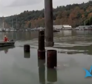
Full-scale mandrel being removed from a driven pile. Note the shoe at the base of the mandrel.
In this video at 2:37, grad student Tim Dardis provides another perspective on the lower end of the mandrel and the shoe as he creates a sub-scale model.

Inserting a sub-scale pile into the lathe. Not sure if this is an outer pile, or an inner pile that is welded to the shoe to create the mandrel. Based on the diameter, I’m guessing inner.

The sub-scale shoe being turned on the lathe. It looks like they are creating a conical surface that will parallel the conical tip of a standard pile.
The mystery in the exciting story is “where’s the spring?”  Per says it is a “flexible coupling” at the bottom of the mandel.  In the lathe video, Tim mentions that the shoe is welded on to the inner pile.  The PBS footage includes short clips of a couple piles on the (Tacoma testing?) dock, as well as a prototype that represents the best public estimate of how the coupling, or shoe, is engineered.
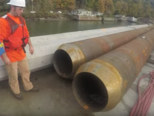
Full-scale piles on the dock. Is the left one the inner pile (mandrel) and the right a standard pile?
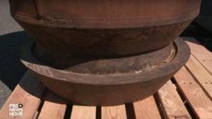
Base of a prototype of the Reinhall pile. Â Where’s the spring?
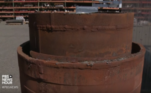
Top of a prototype of the Reinhall pile.
It’s not clear to me where the spring is in this invention. Â But the physics of springs does suggest that the basic idea is a good one (at least for nearby fish, but maybe not for actually overcoming the resistance of seafloor sediments to an inserted vertical pipe).
When a rod-spring system is hit on the top of the rod by an instantaneous force, what happens?  The impact on the end of the rod generates a compression wave that propagates down the rod and eventually compresses the spring a distance which is proportional to a spring constant.  Along the way, energy is transmitted to the adjacent air and through the spring to the sediment.
The dynamics of compressing the spring seem likely to reduce the peak-to-peak amplitude of the compression wave (and pursuant Mach waves in the water and sediment), but isn’t that maximum compression also important in driving the piling through the sediments (which are resisting the driving through friction)? Â Perhaps the acoustic reductions outweigh any loss of efficiency in the driving process? Â One should be careful to not increase sound exposure levels inadvertently — by reducing the noise level but increasing the number of strikes required to drive the pile to the desired depth…
So, how exactly is it put together?  The patent for “Pile to minimize noise transmission and method of pile driving” provide some answers.  First, it suggests that there may be some compliant material used between the inner and outer piles to keep them aligned — at least near the top, and possibly throughout the air-filled void (especially if there are leaks and it fills with water!).
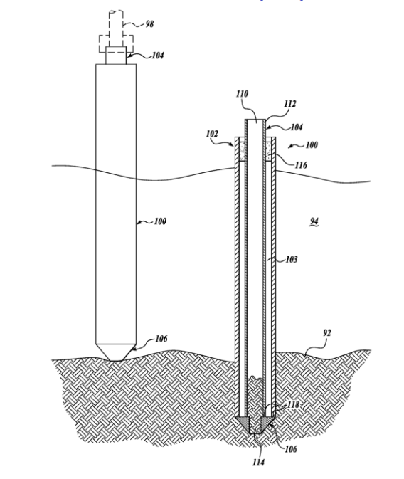
Overview diagram from the schematic. Compliant material (116) helps pile alignment at the top. The driving shoe (106) at the bottom has: an outer diameter equal to or greater than the outer pile’s outer diameter; and, a central aperture (114) to admit sediment with a diameter slightly below the inner diameter of the inner pile.
That all makes sense, but where is the “very, very stiff spring” that’s modifying this massive compression of the inner pile as it reaches the “flexible coupling” at the bottom? Â I thought for sure Fig. 5 of the patent would include a spring…
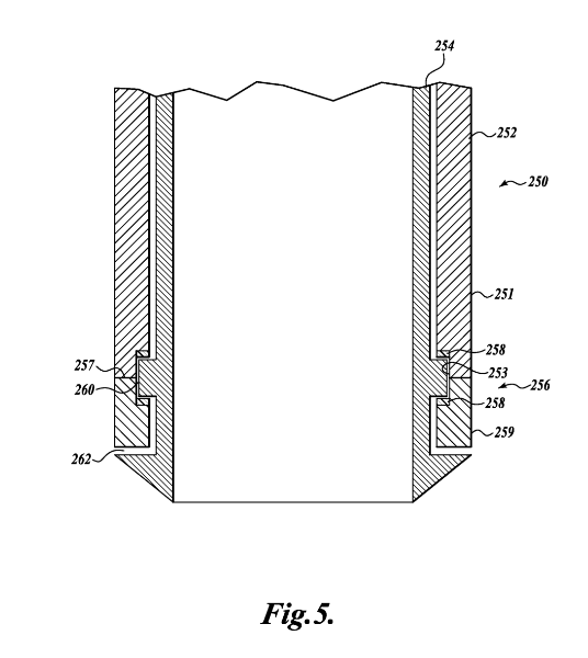
Patent diagram of the inner and outer pile and shoe. Note the flange which connects the inner and outer pile. It pulls the outer pile down behind the shoe as the inner pile is driven. Â I thought 258 would be springs, but no — the patent says “One or two low-friction members 258 (two shown), for example nylon washers, may optionally be provided.”
Still no springs! Â And now the outer pile is welded up so as to “capture” the inner pile. Â I thought the inner pile was going to be re-usable, but now its flange is stuck inside the recess of the outer pile! Â We have, however, got some interesting gaps (260 and 262) separating the inner and outer piles… Â Are we trying to keep water from leaking in?
Maybe, but I don’t get why it’s better acoustically to pull the outer pile down via a flange rather than the aforementioned shoe. Â Maybe the compressional wave transmits less energy to the sediment if it is partially reflected by the flange/recess interface?! Â To me it doesn’t seem worth losing the re-use of the mandrel.
Finally, in the last schematic of the patent (Fig. 6, below) co-inventors Per and Peter (Dahl) of the Applied Physics Lab mention an “elastic connector 285 connecting the inner tube and outer tube” — possibly a spring! Â They suggest it may be “an annular linear elastic spring member with an inner edge fixed to the inner tube 284, and an outer edge fixed to the outer tube 282.”
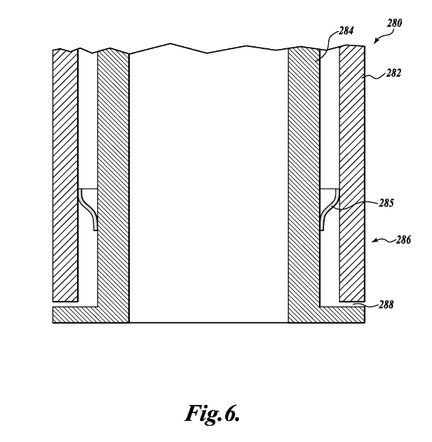
At last a spring! Â 285 is an “annular linear elastic spring member.”
Of course this drawing is a little confusing. Â How are you going to get the inner pile out? Â It seems this also is a non-reusable mandrel “embodiment” of the design. Â And what is 288? Â Mysteriously, it’s not defined in the patent!
No matter how exactly it works mechanically, the invention is effective acoustically.  Overall, the underwater noise is reduced about 20 dB lower (peak-to-peak, or RMS) with the Reinhall pile compared to received levels from a standard pile.  Per explains in the PBS piece that this is equivalent to a 90% reduction in volume (pressure amplitude).  A 20 dB reduction also means the noise is 100 times less intense.
Accolades to the UW and Marine Construction Technology for providing the public with a nice audio clip allowing comparison of the received sound from the control and the Reinhall pile. Â Have a listen!
I’m left wondering who reviews and approves these pretty nebulous patents. Â It seems the design challenge is to optimize acoustic mitigation with efficient installation of the pile — and ideally a pretty standard pile (to save costs and installation steps).
The real innovation of Per and Peter is that they found a way to extend that cylinder of sound-absorbing air down into the sea — not only to the seafloor to block propagation directly in the water (per their ASA talk “Attenuation of pile driving noise using a double walled sound shield”), but also within the seafloor, thereby reducing transmission from the walls of the inner pile to the sediment.  Some of their thought process is captured in this article.
To leverage their good idea within the design constraints I assume, here’s my suggested embodiment:
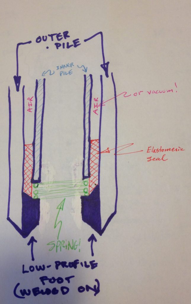
It actually has a big, stiff spring! And:
- minimizes the preparation of the outer pile — just weld to the inner wall of a standard hollow pile a single annular shoe (solid purple) with bevel to guide placement of the inner pile on a driving surface
- seals the connection between the inner and outer pile (to ensure water does not displace the air)Â with an elastomeric material (red) that has a beveled lower edge that weds to the shoe’s bevel.
- Â welds a spring (green) to the base of the inner pile which rests on the driving surface of the outer pile
Read More
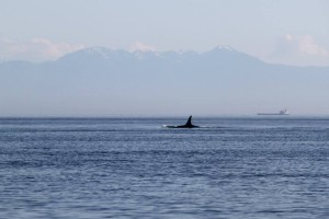
With transient killer whales in the area and the whereabouts of J and L pods (and their many newborns!) unknown, we were concerned to hear that active sonar was utilized late in the morning on Wednesday, January 13, in Haro Strait — critical habitat for species in both Canada and the U.S. At the same time, military training activities were planned or taking place on both sides of the border. This is what it sounded like underwater along the western shoreline of San Juan Island —
Audio Player
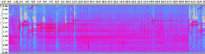
Complex sonar sequence recorded in Haro Strait on 1/13/2016 via the Orcasound hydrophone (~5km north of Lime Kiln State Park).
When the sonar was heard and recorded by members of the Salish Sea Hydrophone Network the Canadian Naval vessel HMCS Ottawa was observed (via AIS) transiting Haro Strait in U.S. waters about 10-20 km north of the hydrophones.
This juxtaposition led us to initially assert that the Ottawa — a Halifax class frigate which carries active sonar — was the source of the sonar pings, reinforced by the activation of the test range (area Whiskey Golf off Nanaimo) on 1/12 and 1/14. However, a proactive call to Beam Reach on 1/14/16 from Danielle Smith, Environmental Officer for Canadian Forces Base Esquimalt, suggested that the Ottawa was not the source. Specifically, she stated that active sonar use was not in their plan when they last departed. She also said she spoke directly with the Ottawa’s Commanding Officer who confirmed with the crew that the transducers were not lowered, and that therefore there was no way their SQS-510 (medium frequency search sonar system) could have transmitted (e.g. sometimes calibrations underway go unreported). Finally, she communicated that their senior sonar techs were confident that the recorded frequencies were not consistent with the Ottawa’s 510 system. When asked, she confirmed that the sonar system had not been upgraded since it was last recorded during the 2012 vent in which the Ottawa disturbed and possibly damaged the endangered Southern Resident Killer whales.
Other sources of information also suggest that the U.S. Navy may have been the source of the sonar pings.
First and foremost, the sonar pings are distinct from the active mid-frequency SQS-510 sonar used by the Ottawa in February, 2012. Instead, they sound similar to, but are more complex than the SQS-53C pings emitted by the U.S. destroyer Shoup on May 5, 2003. [They were also coincident with many individual broadband pings spaced about 6.6 seconds apart. Were these made by the vessel with the active sonar, or a different one?]
Furthermore, comparison of the times of the recorded sonar pings and available AIS tracks suggests that the sonar was recorded when the Ottawa was located between the north Henry Island and Turn Point at the northwest tip of Stuart Island. If the source was the Ottawa, why would it have utilized sonar only while within U.S. waters (about 1-2 km east of the International Boundary). During this period, the Ottawa was about 8-16 km north of the recording hydrophones. Pending computation of the calibrated received levels, the qualitative intensity of the received pings suggests that the source was closer than the Ottawa’s AIS positions allow.
Smith’s statements and these observations raise a key question:Â were U.S. vessels in the area emitting these sounds that are similar to those emitted by the US destroyer Shoup in 2003?
This possibility is alarming because the U.S. Navy has refrained from training with active sonar within the Salish Sea since the Shoup sonar incident of 2003 (which disturbed endangered Southern Residents, as well as a minke whale and harbor porpoises). (The U.S. Navy has tested sonar since the Shoup incident: during the San Francisco submarine event of 2009 and the Everett dockside event in 2012.) Also, the U.S. Navy more recently has agreed to minimize the impacts of its mid-frequency sonar.
Portending a worrisome trend, at the start of 2016 news surfaced that the U.S. Navy planned operations in the Pacific Northwest that might include “mini-subs” and beach landings beginning in mid-January, 2016. No recent AIS tracks of US military vessels have been archived by marinetraffic.com, suggesting that the Navy vessels’ AIS transceivers may have been turned off based on their mission.
Visual observations demonstrate that U.S. Naval ships were active on 1/13/20016. At least one U.S. Naval ship, possibly a frigate, was seen departing Everett around mid-day by Orca Network. Slightly earlier, between 10:30 and 11:30 a.m Howard Garrett of Orca Network saw two Navy ships transiting northward up Admiralty Inlet about 15 min. apart. The first one looked like the Shoup, complete with the cannon on the bow; the second looked more like a supply ship.
(1/17/16 update: A citizen scientist observed two Naval ships southbound in Haro Strait between Turn Point and D’Arcy Island at around 10:45 a.m. — roughly coincident with the sonar heard on the nearby Orcasound hydrophone. 1/19/16: Navy Region Northwest has confirmed a U.S. Naval ship was “in the area…”)
Update 1/22/16: Navy Region Northwest Deputy, Public Affairs, Sheila Murray stated in an email to Beam Reach,
“A U.S. Navy DDG was transiting within the Strait of Juan de Fuca on the U.S. side of the waterway (not in or near the Haro Strait). The DDG confirmed sonar use consistent with recordings on the Beam Reach Facebook page for a brief period of time, approximately 10 min. There were trained lookouts stationed during this event. No marine mammals were sighted during the activity and no marine mammal vocalizations were detected by passive acoustic monitoring. The ship was briefly operating its sonar system for a readiness evaluation in order for the ship to deploy in the near future.”
It is not clear whether the DDG (Guided Missile Destroyer) was one of the Everett-based ships — the Shoup or Momsen — or if it was based elsewhere (e.g. one of the 15 destroyers stationed in San Diego). [Update 1/25/2016: Navy Region Northwest has, however, re-directed a question from Beam Reach regarding the procedures followed by the ship to the Third Fleet (based in San Diego) suggesting that the DDG may have been based in California.]
Update 2/4/16: Lt. Julianne Holland, Deputy Public Affairs Officer Commander, U.S. Third Fleet responded to a question posed by Beam Reach,
Below is the response to your question: Did the DDG obtain permission from the Commander of the Pacific Fleet in advance of this use of MFAS in Greater Puget Sound?
The Navy did not anticipate this use within the Strait of Juan de Fuca. The use of sonar was required for a deployment exercise that was not able to be conducted outside of the Strait due to sea state conditions. The Navy vessel followed the process to check on the requirements for this type of use in this location, but a technical error occurred which resulted in the unit not being made aware of the requirement to request permission. The exercise was very brief in duration, lasting less than 10 minutes, and the Navy has taken steps to correct the procedures to ensure this doesn’t occur again at this, or any other, location. The Navy also reviewed historical records to confirm this event has not occurred before and was a one-time occurrence within the Puget Sound/Strait of Juan de Fuca. The Navy reported the incident to NMFS and NMFS determined that no modifications to the Navy’s authorization are needed at this time.
Below is a chronology of events, wildlife sightings, and acoustic analysis that we hope will help document the event, including the source of the sonar and any impacts on marine life of the Salish Sea.
Key events (local time, PST):
Tue 1/12/16 14:30 PST: Ottawa in search pattern all afternoon and night (1-7 knots, east of Constance Bank)
Wed 1/13/16 09:00 PST: Ottawa moves north into Haro Strait
Wed 1/13/16 10:00 PST: Ottawa enters U.S. waters between False Bay and Discovery Island, proceeds north
Wed 1/13/16 10:45 PST: Intense sonar pings recorded on the Orcasound hydrophone (originating from a U.S. destroyer in the Strait of Juan de Fuca)
Wed 1/13/16 11:00 PST: Ottawa leaves U.S. waters near Turn Point, Stuart Island
Detailed Chronology (public Google spreadsheet):
Acoustic recordings and analysis
8 minute recordings from Lime Kiln and Orcasound
Jeanne Hyde provided 2 recordings — each about 8 minutes long — of a sequence of sonar pings. The first is from the Lime Kiln lighthouse hydrophone (but we believe there is some drift in the time base, so this recording should not be used to assess event timing, like sonar initiation, duration, or ping intervals) —
Lime Kiln 8-minute recording (10:41)
Audio Player
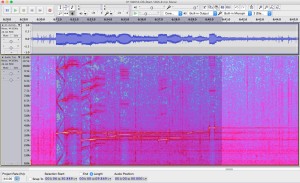
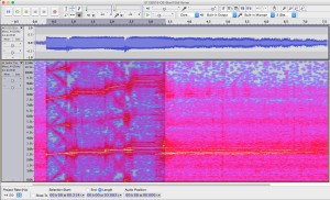
Spectrogram of 8-minute recording from the Lime Kiln hydrophone.
— the second is from the Orcasound hydrophone (about 5 km north of Lime Kiln) —
Orcasound 8-minute recording (10:55)
Audio Player
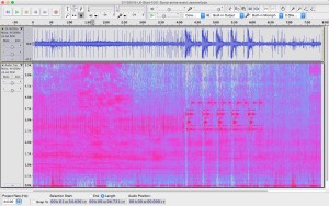
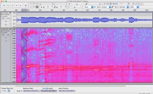
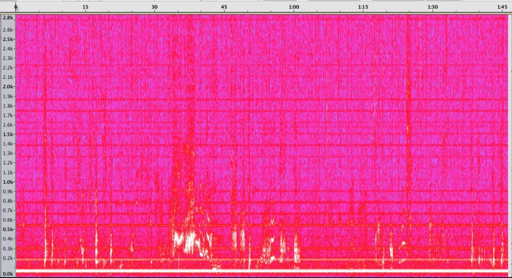
Spectrogram of 8-minute recording from the Orcasound hydrophone.
Assuming that drift in the Lime Kiln recording has corrupted its time base, we use the Orcasound to establish timing of the event. Overall, the event consists of a pattern of broadband pulses and ~30-second sequences of frequency modulated (FM) slide and narrowband continuous wave (CW) pulses. The ~9-minute pattern was: two simple, ascending FM+CW sequences, 52 broadband pulses (2.5-3.0 kHz) about 6.7 seconds apart, and then 5 more FM+CW sequences.Â
The initial and final FM+CW sequences were distinct. The first two were relatively simple and consisted of: a 2.5-2.6 kHz rise for ~0.5 seconds, 2.75 kHz tone for ~1 second, another 0.5 second rise from 2.85-2.95 kHz, and finally a 3.1 kHz tone for ~1 second. The more complicated sequence that is repeated 5 times at the end of the sonar event (around 11:00-11:03 a.m.) is described below (in the section that makes a comparison with SQS-53C sonar sequences emitted by the Shoup in 2003).
The broadband pulse echoes were audible and were received on average 3.4 seconds after the direct path pulse. This time delay indicates a mean extra distance traveled of about 5 kilometers, though there was a clear trend from about 5.7 to 4.4 km over the course of the 52 pings.
Further quantitative analysis of the acoustic data is included in the 13 Jan 2016 sonar chronology Google spreadsheet. The larger data files are archived and shorter clips and associated spectrograms are embedded below.
Sonar sequence repeated 5 times around 11:00
Below is a 2-minute recording of the Orcasound hydrophone (by another hydrophone network citizen scientist) at 11 a.m. on 1/13/16 containing 4 sonar ping sequences. Each sequence lasts 30 seconds and contains a series of complex rising tones followed by single 3.75 kHz tones at about 9 and 22 seconds into the sequence.
Audio Player
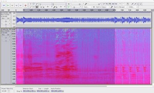
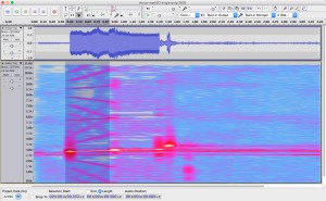
Spectrogram of the final 4 repetitions of the more complex sonar sequence.
Spectrogram showing the detailed pattern of sounds during one of the more complex sonar sequences.
Individual sonar ping at 10:55
Recorded and provided by Jeanne Hyde, this ascending sonar sequence is relatively simple —
Audio Player
Spectrogram of a single ping on the Orcasound hydrophone at 10:55 a.m.
Individual sonar ping at 11:00 (1:14 into ~2hr 26 min recording)
In comparison, this recording (provided by Jeanne Hyde) captures one of the more complex sonar sequences —
Audio Player
Spectrogram of 0.5 second sonar pings at 3.25, 6.5, and 9.75 kHz recorded on the Orcasound hydrophone.
Comparison with SQS-53C sonar pings from 2003 Shoup event
This historic recording from 2003 is similar (relatively abbreviated) to the single ping at 10:55 —
Audio Player
Spectrogram of a single ping from the SQS-53C sonar during the 2003 Shoup incident.
In comparison, here’s one of the more complex sonar sequences observed on 1/13/16 —
Audio Player
Complex sonar sequence recorded in Haro Strait on 1/13/2016.
Overall, the ~10-second sequence has fundamentals and pure tones are between 2.5-3.75 kHz. This makes it distinct (lower frequencies) from the 6-8 kHz tones of Canadian SQS-510 system.
The initial 0.5-second tone has fundamental at 3.20 kHz rising to 3.35 kHz, with intense harmonics at 6.43-6.60 and 9.60-9.90 kHz.  This is followed by a 1.0-second pure tone at 3.45 kHz.
A second 0.5-second tone rises from 2.50-2.63 kHz, with a weak first harmonic at 5.0-5.2 kHz and a moderately intense second harmonic at 7.5-7.8 kHz. This is followed by a 1.0-second pure tone at 2.73 kHz.
There’s a third pair of rising and pure tones at intermediate frequencies, followed by a pause for reverberations/listening, and then a repeat (at lower source level?) of the second and initial phrases. Finally, there is an ending 0.5-second pure tone at 3.75 kHz.
Ship tracks and descriptions
The Canadian frigate Ottawa was observed in Haro Strait at the time of the sonar pings. If the time of the recordings and AIS locations are accurate, then the Ottawa was approximately 8-16 km north of Lime Kiln and Orcasound when the sonar sounds were recorded at those hydrophone locations.
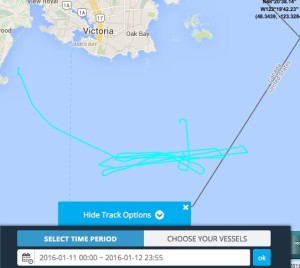
AIS track of the Ottawa on 1/11 to 1/12.
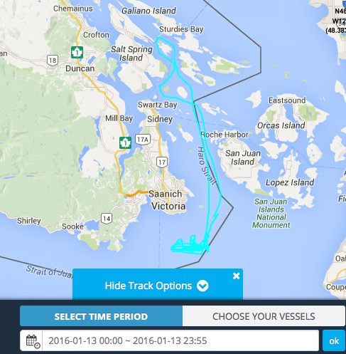
AIS track of the Ottawa on 1/13.
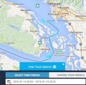
AIS track of the Ottawa on 1/14.
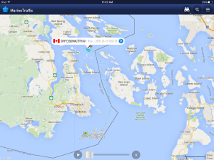
Alternative Ottawa track map
The Canadian Orca class patrol vessel, Caribou 57, was also active and tracked on AIS. From Tuesday 1/12 noon through 1/13 it was patrolling withing the southern Gulf Islands.
Track of the patrol vessel Caribou 57 on 1/12-13.
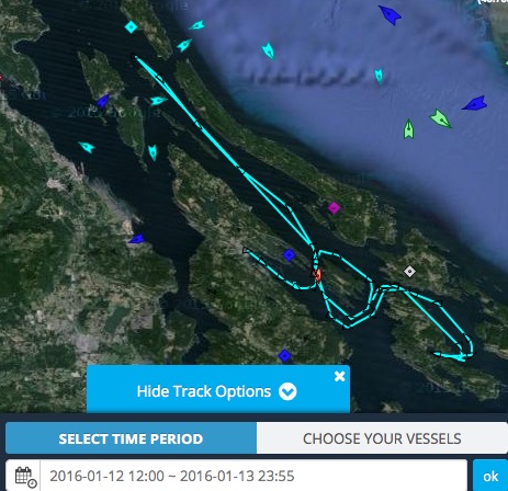
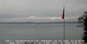
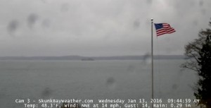
Possible US Naval ships in/outbound from Everett on 1/13/2016 (Skunk Bay web cam):
Read More
NOTE: Due to new information provided by the Canadian Navy, this post has been archived.
A new version with the most up-to-date and accurate information is available here — http://www.beamreach.org/2016/01/14/navy-starts-2016-pinging-in-the-pool
With transient killer whales in the area and the whereabouts of J and L pods (and their many newborns!) unknown, we were concerned to hear that active sonar was utilized late in the morning on Wednesday, January 13, in Haro Strait — critical habitat for species on both sides of the border. At the same time, military training activities were planned or taking place on both sides of the border. At the time the sonar was heard and recorded by members of the Salish Sea Hydrophone Network the Canadian Naval vessel HMCS Ottawa was transiting Haro Strait in U.S. waters.
This juxtaposition led us to initially assert that the Ottawa — a Halifax class frigate which carries active sonar — was the source of the sonar pings, reinforced by the activation of the test range (area Whiskey Golf off Nanaimo) on 1/12 and 1/14. However, a proactive call to Beam Reach on 1/14/16 from Danielle Smith, Environmental Officer for Canadian Forces Base Esquimalt, suggested that the Ottawa was not the source. Specifically, she stated that active sonar use was not in their plan when they last departed. She also said she spoke directly with the Ottawa’s Commanding Officer who confirmed with the crew the transducers were not lowered, and that therefore there was no way their SQS-510 (medium frequency search sonar system) could have transmitted (e.g. sometimes calibrations underway go unreported). Finally, she communicated that their senior sonar techs who said the recorded frequencies were not consistent with the Ottawa’s 510 system. When asked, she confirmed that the sonar system had not been upgraded since it was last recorded during the event in 2012 in which the Ottawa disturbed and possibly damaged the endangered Southern Resident Killer whales.
Other sources of information also suggest that the U.S. Navy may have been the source of the sonar pings.
First and foremost, the sonar pings are distinct from the active mid-frequency SQS-510 sonar used by the Ottawa in February, 2012. Instead, they sound similar to, but are more complex than the SQS-53C pings emitted by the U.S. destroyer Shoup on May 5, 2003.
They were also coincident with many individual broadband pings (classic submarine-movie ones) spaced about 6.6 seconds apart. Were these made by the vessel with the active sonar, or a different one?
Finally, comparison of the times of the recorded sonar pings and available AIS tracks suggests that the sonar was recorded when the Ottawa was located between the north Henry Island and Turn Point at the northwest tip of Stuart Island. If the source was the Ottawa, why would it have utilized sonar only while within U.S. waters (about 1-2 km east of the International Boundary). During this period, the Ottawa was about 8-16 km north of the recording hydrophones. Pending computation of the calibrated received levels, the qualitative intensity of the received pings suggests that the source was closer than the Ottawa’s AIS positions allow.
Smith’s statements and these observations raise a key question:Â were U.S. vessels in the area emitting these sounds that are similar to those emitted by the US destroyer Shoup in 2003?
This possibility is alarming because the U.S. Navy has refrained from training with active sonar within the Salish Sea since the Shoup sonar incident of 2003 (which disturbed endangered Southern Residents, as well as minke whale and harbor porpoises). (The U.S. Navy has tested sonar more recently, however, during the San Francisco submarine event of 2009 and the Everett dockside event in 2012.) Also, the U.S. Navy more recently has agreed to minimize the impacts of its mid-frequency sonar.
Portending a worrisome trend, at the start of 2016 news surfaced that the U.S. Navy planned operations in the Pacific Northwest that might include “mini-subs” and beach landings beginning in mid-January, 2016. At least one U.S. Naval ship, possibly the destroyer Shoup, was seen departing Everett around mid-day by Orca Network. No recent AIS tracks of US military vessels have been archived by marinetraffic.com, suggesting that the Navy vessels’ AIS transceivers may have been turned off based on their mission.
Below is a chronology of events, wildlife sightings, and acoustic analysis that we hope will help document the event, including the source of the sonar and any impacts on marine life of the Salish Sea.
Rough Chronology (local time, PST):
Tue 1/12/16 14:30 PST: Ottawa in search pattern all afternoon and night (1-7 knots, east of Constance Bank)
Wed 1/13/16 09:00 PST: Ottawa moves north into Haro Strait
Wed 1/13/16 10:00 PST: Ottawa enters U.S. waters, proceeds north
Wed 1/13/16 10:45 PST: Intense sonar pings recorded on the Orcasound hydrophone
Wed 1/13/16 11:00 PST: Ottawa leaves U.S. waters near Turn Point, Stuart Island
Detailed Chronology (public Google spreadsheet):
Acoustic recordings and analysis
Sonar sequence repeated 4 times around 11:00
Below is a 2-minute recording of the Orcasound hydrophone (by another hydrophone network citizen scientist) at 11 a.m. on 1/13/16 containing 4 sonar ping sequences. Each sequence lasts 30 seconds and contains a series of complex rising tones followed by single 3.75 kHz tones at about 9 and 22 seconds into the sequence.
Audio Player
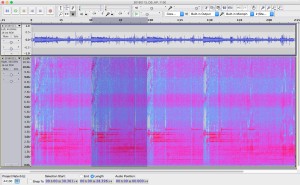
Spectrogram of a sonar sequence that repeated 4 times around 11 a.m.
Spectrogram showing the detailed pattern of sounds during a single 30-second sonar ping sequence.
Individual sonar ping at 10:55
Recorded and provided by another hydrophone network citizen scientist:
Audio Player
Spectrogram of a single ping on the Orcasound hydrophone at 10:55 a.m.
Individual sonar ping at 11:14
Recorded and provided by another hydrophone network citizen scientist:
Spectrogram of 0.5 second sonar pings at 3.25, 6.5, and 9.75 kHz recorded on the Orcasound hydrophone.
Comparison with SQS-53C sonar pings from 2003 Shoup event
Audio Player
Spectrogram of a single ping from the SQS-53C sonar during the 2003 Shoup incident.
Ship tracks and descriptions
The Canadian frigate Ottawa was observed in Haro Strait at the time of the sonar pings. If the time of the recordings and AIS locations are accurate, then the Ottawa was approximately 8-16 km north of Lime Kiln and Orcasound when the sonar sounds were recorded at those hydrophone locations.
AIS track of the Ottawa on 1/11 to 1/12.
AIS track of the Ottawa on 1/13.
AIS track of the Ottawa on 1/14.
Alternative Ottawa track map
The Canadian Orca class patrol vessel, Caribou 57, was also active and tracked on AIS. From Tuesday 1/12 noon through 1/13 it was patrolling withing the southern Gulf Islands.
Track of the patrol vessel Caribou 57 on 1/12-13.
Possible US Naval ships in/outbound from Everett on 1/13/2016 (Skunk Bay web cam):
Read More
I’m giving a talk on our recent paper (PeerJ Preprint) at the Green Tech Conference in Seattle today. Here is the agenda and my presentation:
And some notes I took during the 2-day conference in downtown Seattle.
 Introduction
Green Marine is a non-profit based in Quebec, Canada, that certifies environmentally sustainability in the shipping industry. The initiative has a growing number of Canadian and U.S. ports [Seattle, Long Beach, New Orleans] and has 50 supporters (NGOs [including Seattle-based Puget Sound Clean Air Agency, Seattle Aquarium]. The number of participating organizations is growing (about 66% increase between 2013 and 2014). Green
Panel presentations and discussion
SUSTAINABILITY AT WORK IN MARINE TRANSPORTATION MADISON
- Linda Styrk, Managing Director, Seaport Division, Port of Seattle
- Stephen Edwards, CEO, GCT Global Container Terminals Inc.
- Dennis McLerran, Administrator, U.S. EPA Region 10
Linda:
The Century Agenda is the Port of Seattle’s 100-year vision: to be the cleanest, greenest port in North America. The Green Marine certification program emerged as the best way to progress environmentally. Stefanie Jones Stephens is Environmental Manager guides performance in different Green Marine metrics.
One practical example of the utility of the certification metrics is comparison with other ports and standards. The Port was surprised to score low in the in-air noise metric because few complaints had been received (possibly due to their proactive outreach). Quantitative comparison made it clear that an improvement could be made.
She showed videos of run-off filtering tanks (Harbor Island) and experimental above-ground gardens (“SplashBoxes” in areas where digging isn’t possible) for decreasing water pollution. In a project managed by GeAlogicA and funded by the Seattle Foundation, Capital Industry built rolling containers that held volcanic soil and plants. Port developed grant program (~$30,000-50,000 assistance to each participating truck/owner) that helped replace 500 trucks to reduce pollution during the 2000 truck trips per day.
Overarching thought is that the marine industry is very innovative, but perhaps too low-profile about it’s environmental advances. The Port of Seattle has many other green innovations (biodiesel, stack-scrubbers, …), but too few members of the public know about them.
Stephen
Container terminals (warehouse w/o roof!) are a distinct operation (e.g. from bulk facilities). GCT is based in Vancouver owned by a pension fund in Canada with U.S. terminals in New York and Bayonne. We consider ourselves a technological leader that serves 19 out of 20 global container shipping companies.
We didn’t know how we compared with other organizations in our industry. Green Marine was chosen because its metrics are driven by the participating organizations, not our customers.
There is an industry shift to larger vessels. Same number of ships, less weekly trips, and fewer companies. TEU has nearly doubled in 10 years (~2003-2013). Europe and Asia are seeing up to 20,000 TEU ships now…
Vessel sharing agreements group shipping companies (e.g. Maersk) into only 4 “customers.” North American Emissions Control Act caused higher costs in coastal waters (and therefore quicker turn-arounds): cleaner burning fuel costs 600$/ton vs $400/ton in the open ocean. These changes motivate investments in ship-terminal-truck semi-automation, scheduling, worker safety, and other logistics (e.g. no idling during waits).
Dennis (used to work for Puget Sound Clean Air Agency)
EPA has worked with 159 countries and the IMO to develop a uniform fuel requirement through the North America “ECA” (pronounced “Eek-uh” = Emissions Control Act requires large vessels to use cleaner fuel within 200 nautical miles of the coast). This rule prevents 31,000 premature deaths, 1.4 M loss work days, as well as lost school days (through the connection between ship exhaust and human health).
EPA is committed to working with the industry to find innovations that benefit the environment as well as the bottom line. Some examples of mutually-beneficial partnerships with industry. EPA worked with Tacoma-based Tote (RoRo line) is converting ships to burn (non-distiallate) cleaner fuels or LNG, which in the long-term will reduce cost of consumer goods in Alaska. Diesel Emissions Reduction Act (DERA funding, RFP due June 15) has reduced pollution while returning value to the U.S. Government (usually through reduced human health costs). The SmartWay programs helps partners move more goods for reduced cost, in part by building off EPA’s brand equity.
EPA is developing a national port initiative, building off experience and leadership (of CA Ports). The key is for Ports to realize that they are stronger when both providing services to their customers and keeping their local communities and workers healthy.
 10:30 session
TECHNOLOGY GEARED TOWARDS REGULATORY COMPLIANCE: LESSONS LEARNED
4 talks:
- Emissions scrubbers on the Algoma Equinox class vessels (Mira Hube)
- These ships are more fuel efficient and have reduced water use and noise pollution.
- We operate in emissions control area 100% of the time, so needed to reduce sulfur emissions (and NOx and particulates)
- LNG was an options, but there is a lack of LNG infrastructure in the Great Lakes
- EGCS
- Overview of exhaust gas cleaning system (EGCS)
- Manufactured by Clean Marine (Norway)
- Closed-loop, fresh water, NaOH scrubber
- Base neutralizes acidic emission components;effluent is treated onboard, then discharged
- CSL’s Experience with Ballast Water Management Systems (BWMS) (Yousef El Bagoury; and Kevin Reynolds from Glosten Associates)
- How do you choose a BWMS?
- 70+ on market; 32 IMO-approved; 16 have USCG temporary approval…
- Glosten did early BW installations in 2006, so helped evaluate options
- Glosten worked with CSL to 3D laser scan possible sites in CSL ships
- How to fit (massive) pumps (2k m^3/hr!); heaters; hydrogen vents; filters?
- 3D models and equipment size guided plans for shipyard installation
- Lessons learned
- Lots of (EPA/USCG) paperwork involved in permits and Class approvals
- Site supervision and crew training are critical
- Clean ballast tanks prior to commission (ours had mud that clogged filters)
- Preparing for USCG approval (testing late summer, 2015)
- Other ships getting 3D scans by Glosten
- Saga Forest Carriers – Ballast Water Treatment (BWT) Case Study (Birgir Nilsen)
- Optimarin started as ballast water treatment company in 1990s.
- 225 systems at sea; 50 are in use (on bulk carriers, Naval vessels…); medium scale — up to 3000 m^3/hr (largest are 7000 m^3/hr, e.g. in cruise ships)
- Regulatory environment: IMO, but also USA (USGS National Invasive Species Act; EPA Clean Water Act; plus confusing State variants (e.g. CA, Great Lakes))
- Pre-market conditions: customer buys equipment and intallation through “type approval certificates” (which should specify limits, like UV transmission and/or temp/salinity…)
- Basic system filters first and then disinfects with UV light (up to 35 kW from single lamp!)
- Sage Forrest Carriers (Optimarin customer)
- Open hatch mostly in paper pulp trade
- 1-2 km^3/hr ballast flows
- 3D scans (through Goltens sub-contract) of 24 ships (4 different ship designs)
- Little to no space: used part of ballast tank for equipment!
- System successful, but key is user training and operation manual (via officer conferences)
- Membrane Scrubber Technology for SOx Removal from Engine Exhaust (Gerry Carter & Edoardo Panziera)
- Wet scrubbers (dry scrubbers are used on land, but takes too long to warm up/down & maintain)
- All designs use combinations of sprayers and filters and (Achilles heel) water treatment systems
- Ionada innovation is a ceramic membrane separation technology
- Provides surface area for the chemical reactions (resulting in a clean crystal)
- But without mixing with the exhaust gases
- No PAH wastewater treatment!
- Potassium carbonate is less toxic than NaOH; reacts with SOx to from K2CO3 (a fertilizer).
- $14 to purchase KCO3; $14 from sale of fertilizer!
1330 session
CORPORATE ENVIRONMENTAL LEADERSHIP: INSPIRING INITIATIVES FOR THE INDUSTRY
Cooperation between NGOs and Industry to Define Sustainable Development in the Canadian Arctic
Andrew Dumbrille, WWF Canada & Marc Gagnon, Fednav
- FedNav (Marc)
- Canada’s largest dry cargo shipping group
- 1/3 grain, 12% steel, 14% alumina, 17% industrial mineral
- 80 ships: 59 operating, mostly handysize (Lakers), but more and more supramax and ultramax ships
- 24 ships on order, growth in part developing Arctic (Baffinland iron ore; Red Dog AK zinc/lead)
- Has environmental policy
- Working with WWF since 2011 (Marc)
- chosen due to being leader in industry, only company in Arctic during winter
- shared vision signed 2013
- What does it take to work with an NGO? Patience!
- Shared goals: environmental; economic; polar guidelines
- Completed “Best Practices in the Arctic” document
- Challenges: goals are different! Different positions on Arctic shipping (LNG only initiative is economic folly). Other WWF partnerships are sometimes in conflict with FedNav collaboration.
- WWF (Andrew)
- 5M members, 5000 staff, 500 million raised
- Hudson Strait: Reducing shipping impacts & risks (May 2015 contract report by Vard Marine, funded by FedNav)
- Key recommendation was a Polar Shipping Operating Manual (e.g. marine mammal behavior, set-backs, etc.)
Radical Improvements in Vessel Efficiency
Lee Kindberg, Maersk Line (co-chairing EPA Clean Cargo working group)
- Maersk enables trade with benefits and costs to the planet and humanity.
- 90% of all goods transported globally are carried by ship
- Ocean shipping 4% of global emissions (though NASA map still shows an impact)
- Since 2007, Maersk has been able to grow containers shipped by 40% while lowering CO2 emissions by 25%
- Energy efficiency makes good business sense.
- Using Clean Cargo Working Group metric, mean CO2/TEU/km, levels fell from 70-45% between 2008 and 2013 through new vessels, eco-retrofitting old vessels, “smart steaming” and network design (which ports of call, scheduling, personnel efficiency competitions)
- 2020 goal is 60% reduction
- Voyage Efficiency Systems (communications between leading and following ships) has evolved to Global Voyage Center (in India staffed 24/7 by 10 masters & 10 chief engineers)
- Terminal Efficiency Project: minimize harbor time to reduce local emissions, then slow steam later to regain coastal fuel losses
- New ships higher efficiency and have enormous economies of scale (e.g. Mary Maersk carries ~17.6 kTEU at 2,200 miles/gallon/ton)
- Of three new classes, biggest is Triple E: 18 kTEU, 50% more efficient (in part through waste-heat recovery systems)
- Retrofit options: new bulbous bow (“nose job” helps when vessels that used to run 22-24 knots are running at 16-18), prop, propeller boss cap fin, engine de-rating, fuel flow meters.
- Propeller optimization reduces cavitation
- Committed to $1 billion over 5 years for retrofitting 100 of owned vessels
- Reducing speed to <10 knots in Santa Barbara channel when whales are present… also have reduced speed on Atlantic seaboard (to protect Right whales?)
- Big shippers have played a role in motivating lower carbon shipping initiatives, but so have our core values… as have the economics of increased fuel efficiency in an era of expensive fuel.
ECHO Program: Collaborating to Manage Potential Threats to At-Risk Whales from Commercial Vessels
Carrie Brown & Orla Robinson, Port Metro Vancouver (Environmental Programs Department)
- Enhancing Cetacean Habitat and Observation Program
- Mandate under Canada Marine Act: facilitate trade but in ways that are safe for the environment
- Initiated due to DFO status of species at risk and projected shipping growth
- History
- 2014-15 planning and launch
- 2016-17 development of target and implementing mitigation
- 2017 manage adaptively to reduce threats over time
- Advisory Working Group
- Acoustic Technical Committee: DFO, JASCO, NOAA, ONC, Robert Allan Naval Architects, SMRU, Transport Canada, UBC, U St. Andrews, Vancouver Aquarium, WA State Ferries
- Work plan: acoustic disturbance, physical disturbance, environmental contaminants; timely as in the last month we had a fuel spill in English Bay and a fin whale on a cruise ship bow…
- Acoustic Disturbance focus areas: will include vessel noise “weigh station,” hull cleaning
- Mitigation prospects: green tech, operational management options, criteria for Green Marine performance indicators (ultimately adding noise to air quality EcoAction program)
- Physical disturbance: working with DFO to survey and assess strike risk assessment; whale sighting and notification system; west coast mariner’s guide…
- Environmental contaminants: baseline sampling sediments and mussels, esp during hull cleaning
15:30 session
EMERGING ENVIRONMENTAL ISSUES: AN INTRODUCTION TO UNDERWATER NOISE
Whales in an Ocean of Noise: How Manmade Sounds Impact Marine Life
(Kathy Heise, Vancouver Aquarium)
Early hydrophone work was from lighthouse, small boats, and included interest in Pacific White-sided Dolphins.
Shipping industry should keep in mind role of ship noise in cumulative acoustic impacts on all sound-using marine organisms (with other major sources being pile driving, seismic surveys, and military sonar).
Change is beginning: 2009 letter to Obama; IMO voluntary guidelines for vessel equipment and design (2014); EU Marine Strategy Framework. Good news is that practical solutions are at hand. It may be more expensive initially, but can save money in the long run.
Ship Noise in an Urban Estuary Extends to Frequencies Used by Endangered Killer Whales
(Scott Veirs, Beam Reach Marine Science)
Control and Measurement of Underwater Ship Noise
(Michael Bahtiarian, Noise Control Engineering)
- Ship noise vs shipping noise
- Analogy with aircraft and airports, but aircraft have a service life of 5 years while ships have one of 20-30 years, so quieting may be slower than what occurred in planes in the 1960s and 1970s.
- Research and fisheries have much of the quieting technology (not just the Navies)
- Vessel noise sources: cavitation, machinery,…
- Ship Noise Analysis Software helps establish a baseline and then assess improvements
- Mitigation technologies: insulation; vibration isolation; damping (spray-on and tile versions; from military innovations); floating floors/rooms; bow thruster and HVAC treatments
- Existing benchmarks
- International Council for the Exploration of the Seas (1995) ICES/CRR-209
- applies to fisheries and research vessels
- Followed by Europeans since 1995
- DNV, Silent class, 2010
- various “notations” (grades)
- Notations depend on class
- Measurement standards
- ANSI/ASA S12.64: Established 2009, first standard for UWRN
- Meeting next week to finalize ISO 17208-1: Precision method for deep water
- General methodology (figures from ANSI/ASA S12.64-2009)
- Facilities for UWRN measurements (can be provided to private industry by Navies)
- SEAFAC (Ketchikan, AK)
- Dabob Bay (Seattle, WA)
- San Clement Island (San Diego, CA)
- Florida
- Halifax?
- Noise Control Engineering uses BAMS (Buoy Acoustic Monitoring System)
- UWRN Design Guidance
- SNAME T&R Bulletin, 3-37, “Design Guide for Shipboard Airborne Noise Control,” 1983 (Supl 2000)
- JIP/OGP Report
- SNAME 6-2, MVEP GM-1, Ocean Health and Aquatic Life
- BOEM Report 2014-061
- Pending IMO Guide “Guidelines for the reduction of underwater noise for commercial shipping (estimated to be issued by 2016); a bit of a compromise of US, China, Europe, and (opposing) flag nations like Vanatu
Read More
Thanks to Professor Rick Keil and his UW Oceanography 409 class on Marine Pollution, I had a chance to go back through the data archives and review the research progress made over the last decade by Beam Reach students and faculty. Below is the talk I’m giving today in Rick’s class to wrap up their study of underwater noise pollution in the marine environment.

Read More
While we continue spending this summer analyzing data we’ve collected over the last ~10 years, we’d like to recap what we accomplished last summer. This post is co-authored by Scott Veirs and Beam Reach alum and 2012-2013 intern Breanna Walker.
Bre observing Haro Strait from the Lime Kiln lighthouse.
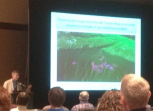
In 2013, Beam Reach collaborated with The Whale Museum and Lime Kiln State Park by maintaining long-term research projects at the lighthouse, and by mentoring a summer intern: Beam Reach alum Breanna Walker. It was Bre’s second summer studying the role of vessels in generating underwater noise and their potential effects on the behavior of Southern Resident killer whales (SRKWs) as they pass by Lime Kiln (Whale Watch) State Park on the west side of San Juan Island (WA, U.S.A.). Here, Bre and Scott provide first a synopsis of our research and education efforts at Lime Kiln during the summer, and then an overview of our long-term research activities at what we like to call the “Lime Kiln Acoustic Observatory.”
Summer 2013 research & education
Despite the fact that SRKW activity was slower throughout summer 2013 than previous years, research and education was in full swing from June through September at Lime Kiln Acoustics Observatory. Bre spent the summer at Lime Kiln waiting for J, K, and L pod to enter Haro Strait in pursuit of salmon. Thanks to Jason Wood of SMRU Ltd. setting up continuous recording of the hydrophones, we were able to obtain a larger sample of early morning and late night SRKW recordings. These 24/7 recordings supplemented the surface behavior observations and vessel monitoring efforts that Bre undertook during daylight hours. Bre also worked with Jason on a project for SMRU Ltd., localizing SRKW calls from the 2012 season to determine their source levels.
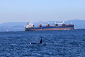
A male Southern Resident and ship sharing the waters of Haro Strait
Summer started off with a bang as there was a lot of whale activity in late May and early June at Lime Kiln as we were expecting.  However, all the early excitement was followed by an abrupt drop in sightings. Anomalously low prevalence persisted in June and continued for the majority of the summer.  After nearly an 11 day stretch with only one sighting of whales, the L22’s (a sub-group of L Pod) provided a unique opportunity for data collection on June 21st and 22nd when they lingered on the west side of San Juan Island for a week or so after the rest of the SRKW population was assumed to have headed back out to the open ocean. The L22 sub-group is composed of the female matriarch L22, and her two sons L89  and L79.
These encounters with the L22s were interesting, not just because it was so unusual to have them isolated from the rest of the population. Often at Lime Kiln we observe the whales “shuffling” either north or south, occasionally pausing to forage, but typically moving along the west side. However, in these encounters the L22s seemed to linger in front of the lighthouse, displaying surface behaviors indicative of foraging, often with the primary acoustic signals being echolocation clicks for extended periods of time, rather than vocalizations. After a few days of this behavior, Bre, along with fellow Lime Kiln Researcher Bob Otis and his interns, began to notice that the whales seemed to head north in Haro Strait shortly before or after the tide changed from flood to ebb. The L22s would leave the southwest end of San Juan Island where they had been sighted spending a lot of time near Eagle Cove and Pile Point, and moved north to the Lime Kiln Lighthouse. This behavior was observed for a few days in June, and then again during the first week of July. Just as we thought we had noticed a pattern they went and did the opposite. However, these less-than-usual encounters got the whale community’s attention and everyone was curious as to why they remained in the area around while the rest of the population was beyond the Salish Sea. Of course, now that L79 has been missing since mid-summer last year (2013), these encounters seem even more intriguing. As we move forward with data analysis, we are especially interested in analyzing the days when only the L22s were present.
The “week of whales” — as it was dubbed by the lighthouse crew — was July 8-12, 2013. During these four days all three pods (a superpod) passed by the lighthouse numerous times. The SRKWs were not sighted again at the lighthouse for another 26 days, with the exception of two encounters with K pod on July 19 and 20. During that time there were two Transient pass-bys, which were recorded during Jason’s data collection for a SMRU project, in which we were recording 24/7.

A juvenile breaching along the west side
The summer continued on in a dry spell of sorts. It seemed that the SRKW spent more time out of Haro Strait than they did in, and when the whales were present on the west side, they did not frequent the lighthouse as often as was expected. As of July 26th, 2013, Bob Otis had documented only 17 whale days, less than 50% of the 35 days recorded as of July 26th, 2012. This pattern continued into the month of August.
Despite the lack of whale activity at Lime Kiln last summer, visitors still frequented the lighthouse. In September, Bre worked as a naturalist for The Whale Museum, educating visitors about the whales, salmon, and the Salish Sea ecosystem. The lack of whale activity at the lighthouse frustrated many visitors, however it opened up great conversations about the ecosystem dynamics and the importance of salmon and clean waters for the whales. Overall, it was an educational field season, sparking both concern and curiosity for the future of the Southern Resident Killer Whales, the salmon, and the rest of the Salish Sea Ecosystem.
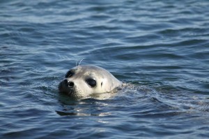
Curious seals frequent the Lime Kiln shoreline
Links to meta/data —
Long-term research progress
Throughout 2013, Beam Reach maintained a Vemco VR2W fish tag receiver as part of a collaborative resident Chinook salmon (black mouth) tracking project with UW & NWFSC. The receiver was deployed adjacent to the long-term Lime Kiln hydrophone using an existing cement mooring anchor. It was serviced by David Howitt & Jason Wood on 9/13/2013 during a dive in which #110849 was recovered (having been deployed on 4/12/2012) and #102782 was deployed. Link to field notes and metadata. While the grant has ended (most San Juan equipment was recovered in late 2013 or early 2014) Beam Reach is helping to analyze the data and is maintaining a VR2W receiver at Lime Kiln in 2014.
Beam Reach helped maintain the calibrated hydrophone system throughout 2013, both to support the Salish Sea Hydrophone Project and to continue measuring received sound pressure levels of passing commercial ships. Although no new funding was available from NOAA in 2013, Beam Reach paid sub-contractor David Howitt to service the bottom-mounted hydrophone.
As part of the ship noise project, Scott and Val collaborated with Jason Wood of SMRU Ltd. Beam Reach supported the archiving of AIS data in 2013 for passing ships with software written by Val Veirs. The data set now encompasses 31 months from Mar 2011 – Oct 2013 and has been analyzed. We are submitting a paper summarizing noise from about 1500 unique ships in spring-summer 2014.
Finally, Beam Reach continued to maintain the live streaming hydrophone system at Lime Kiln with our partners. While the number of entries for Lime Kiln in our citizen science log (97) was only down ~70% from 2012 levels (325), this reduction in one proxy for listening effort was countered by a rise in another — the number of “hearings” reported on the Orca Network Facebook page. An observational highlight of 2013 from the nearby Orcasound node of the Salish Sea Hydrophone Network was humpback vocalizations (feeding calls, according to Jared Towers) heard for the first time in Haro Strait on October 13, 2013 and recorded by Jeanne Hyde.
Audio Player
Audacity spectrogram of first humpback recording from Haro Strait
Unlike in previous years Beam Reach did not deploy other scientific instrumentation at Lime Kiln in part because we did not run spring or fall undergraduate programs in 2013. Pending renewed funding and educational programs, we will continue to propose new studies using: the existing and new live streaming web cam, our cabled underwater video camera, oceanographic instruments, and a thermal imaging camera.
Read More
Thursday, 5/1/2014
8:30
Parker MacCready (with Matthew Alford)
Observations of flow and mixing in Juan de Fuca Canyon
Pacific water on the continental shelf exerts strong control over Salish Sea productivity, hyposia, and acidification. It is the most important source of nutrients for Puget Sound by a couple orders of magnitude.
The problem is that the Pacific water properties vary strongly with depth. There’s high oxygen water near the surface (DO as high as 110 near 150m) and low oxygen water below (DO ~50 at 800m).
The water enters the Strait of Juan de Fuca via the Juan de Fuca canyon, an understudied region
(see Glenn Cannon, 1972) that cuts across the continental shelf. It’s deep enough relative to the shelf that the inflow can move up the canyon (moving east-northeastward at about 40 cm/s, independent of the tidal state) underneath the surface current on the shelf (typically southeastward flow).
The along-canyon flow gets up to 75 cm/s. As it moves over sills, internal lee waves form that have amplitudes of up to 80m.
ROM model runs show inflow across shelf is primarily via the canyon:
Richard Feely
The impacts of upwelling ocean acidification and respiration on aragonite saturation along the WA continental margin
Due to upwelling we are seeing pH conditions that won’t be seen the global surface ocean until the end of this century. The upwelling low O2 water also has high pCO2, low aragonite saturation state, low pH for water >80m depth.
Feely described a new model that can predict water properties 6 months in advance, a tool which could be very valuable to Salish Sea shelfish growers.
Local respiration uses up the (already low) oxygen and increase pH as the water flows in. This can result in anoxic events downstream.
What forces the inflow? Wind from the north!
Ref: Alford and MacCready (2014) Flow and mixing in Juan de Fuca Canyon, Washington. Geophysical Research Letters, 41.
Rob Fatland is talking later about using ROM to visualize the flow of water across the shelf, primarily via the canyon.
The transport observed is about equivalent to the Amazon River, 200,000 m^3/s, easily enough for the Salish Sea “estuarine circulation” about 30,000 m^3/s.
9:00
Christie McMillin (Marine Education and Research Society mersociety.org)
Anthropogenic threats to humpback whales in the Salish Sea: insights from northeastern Vancouver Island
2012 Juvenile humpback stranded (long line entanglement)
2013 photographs (by Mark) indicate that it was a high recent year (along with 2011; nice graph)
1985 Merilees documented two periods of whaling in the Strait of Georgia in the late 1800s. Place names like Blubber Bay reflect this history.
Northeast Vancouver Island had whaling as late as 1968 and many humpbacks were taken in the 1950s on the west side of Vancouver Island.
Since 2006 they have documented 8 vessel strike injuries. Since 2009 there have been 5 witnessed cases of entanglement in prawn gear (3), crab gear (1), and seine net (1). In 4 of 5 entanglements, the whale was disentangled.
We can estimate total (non- + witnessed) entanglements by photographing leading edge of tail stock. This method suggests that 9 additional entanglements have occurred in our study area.
There are concentrations of humpback distributions northeast of Hanson Island, while much lower densities occur in Johnstone Strait (particularly SE of Hanson). This observation informed new signs warning vessel operators of the high density areas.
Is you witness entanglement or ship strike, DFO has a hotline, but with a VHF you can call the Coast Guard.
9:15
Jared Towers (DFO/Marine Education and Research Society)
New insights into seasonal foraging ranges and migrations of minke whales from the Salish Sea and coastal British Columbia
Minkes do breach!

Highest distributions are on west side of San Juan Island, the banks, and Race Rocks, as well as North Vancouver Island. Lower densities further north and on the outer west coast of Vancouver Island. Despite effort, none were observed off Nanaimo area in the Strait of Georgia.
Strong seasonal distribution, peaking in July. No sighting during ~Oct-Mar.
Previous research: Dorsey et al., 1990. Rep Int. Whal. Commn. Special Issue 12.
Intra-annual movements occur spring-to-summer and summer-to-fall suggest migration. Ecological markers (e.g. scars, swordfish beaks embedded in blubber, diatom coatings or barnacles, cookie cutter shark bites, lamprey scars, Xenobalanus colonizing trailing edge of fins [occurs in tropical east Pacific]). Ref: Towers et al. (in press) Cetacean Research & Management (?)
Prey seems to be juvenile herring and juvenile and adult sand lance. We observe bait balls in the NVI and they may occur in the SJI area, too.
9:30
Marla Holt (recording in .mp3 format)
Using acoustic recording tags to investigate anthropogenic sound exposure and effects on behavior in endangered killer whales
Goals: quantify noise that individual SRKWs experience; determine relationship between vessels and their attibutes and received noise levels (RL); investigate kw acoustic and movement behavior during foraging.
Digital Acoustic Recording Tags (DTAGs) have two hydrophones (one for background noises, one for KW signals), as well as orientation and movement sensors. We have 3 field seasons of data so far (Sep 2010 [before 2011 vessel distance increase from 100-200 yards], Jun 2011, Sep 2012) and plan more deployments this year. 23 tags on all three pods.
Animation of a 7-hour tag in Haro Strait SE down Haro canyon, across to Salmon bank, south along its western edge, and then across to ENE Hein bank.
Received levels: RMS averaged over 1 sec in dB re 1 uPa, 1-40kHz band. 2768 measurements of RL (w/o flow noise or whale signals), min 88 dB (3 vessels 2 stationary 1 slow (0-2) kts; Max 141 dB large fast vessel (ferry passing less than 300m from whale!) Julian Houghton’s theses working up predicted noise levels and finding speed and (size, distance??) are most important factors in RL.
Variations in pitch and roll may indicate foraging changes, but few prey samples have been acquired during focal follows with DTAG deployments.
9:45
M. Palomares
The Salish Sea ecosystem in FishBase and SeaLifeBase
We have documented the iodiverstiy of Salish Sea in two databases:
- fishbase.ca
- sealifebase.ca
~82 references used to assign 2,280 species to for ecosystems
Gatydos et al. 2008, 2011; Cowles 2005
Fish completed; birds and marine mammals need work; many invertebrates.
The full fish list is at — http://www.fishbase.ca/trophiceco/FishEcoList.php?ve_code=1067
These data (particularly the trophic pyramid, as well as the “1-click ecosystem routine’) should help researches build ecosystem models. 68% of fish species have biological data in FishBase. There are at least 12 species that are commercially important that don’t have life history data, so they could not be included in the reslience estimations.
There are efforts to cross-reference with the barcode of life movement.
10:45
I. Vilchis
Common risks among declining marine predators suggest ecosystem change
39 taxa of wintering birds in 8 Salish regions and three depth categories
The birds most likely to undergo a decline (based on their model) were the diving birds without local breeding colonies. Across categories, decline probabilities are higher in the birds that eat fish (vs non-fish eaters).
Why are diving birds over-wintering less in the Salish Sea? We suspect that this is because there have been long-term decreases in the forage fish abundance in the Salish Sea. (Some studies have shown concomitant increases in over-wintering populations in California.)
One idea is that the specific power required to maintain a certain air speed is much higher for diving birds. (Nice use of archive.org videos embedded in slide to show difference in flapping frequency in puffins vs frigates.)
Conclusion: Salish Sea birds are shifting wintering feeding ground as a result of lack of prey.
11:00
P. Arcese
A century of change in trophic feeding level in diet specialist marine birds of the Salish Sea
Western Grebes have declined by 97% in 40 years here and increased 230% in southern CA. Pacific sardines were extremely abundant before being overfished, but the have come back dramatically since the 1980s (Ref Hill, 2010?)
Murrelets in BC have gone from ~500k to 50k population and were studied isotopically using historic samples (feathers formed early in year [condition prior to breeding]) from museums around the world, including bird collected by Vancouver (Norris et al. 2007, Journal of Applied Ecology). The dN15 decline they observe suggests a decrease in trophic level of the murrelet diet from mainly fish to mainly euphausids. Fecundity vs bird count data, suggest that forage fish abundance may be limiting reproductive rates.
Even glaucus winged gulls are in decline. Mondarte populations down from ~3000 to ~900. Average age size is also decreasing (Blight, 2011).  The isotopic decline in gull feathers is consistent with the murrelets.
The western grebe is a herring specialist, but isotopic data from grebes have maintained diet (on herring) but most have left the Salish Sea.
11:15
Jessica Lundin
Persistent organic pollutants (POPs) in the Puget Sound ecosystem: An evaluation of POPs in fecal samples of Southern Resident killer whales
247 samples in final analysis, including toxicants, hormones, and genotyping
Toxicant results: dried fecal samples vs blubber samples from same whale (30 whales) show strong corrleation; unprocessed (undried) fecal samples vs blubber also highly correlated.
- Higher ratios of ppDDE/sum(4PCB) are highest in L, and secondarily K pods relative to J pod
- Females with >1 calf have lower 2-5x toxicant loads than juveniles, males, and post-reproductive females (who have the highest values)
Graphs of Columbia and Fraser Chinook returns show a ~2 month gap during which there is evidence that toxicant are being mobilized from their lipid stocks.
Ratio of sum(PBDE)/ppDDE shows an increasing trend (2010-2013) suggesting that PBDEs are bioaccumulating.
Next steps are to look at relationships between toxicants and hormone. A pregnancy test has been developed which could be used to assess reproductive success (and hypothetically may be influenced by toxicants).
11:30
30 minute discussion (.mp3 format) at end of Session on “Marine birds and mammals of the Salish Sea: identifying patterns and causes of change – II”
Lunchtime presentations:
 Friday May 2, 2014
9:30
Natalie Hamel
The 2013 State of the Sound Status of the ecosystem
PSEMP = Puget Sound Environmental Monitoring Program works with partners to monitor and report conditions and assess restoration efforts. The Puget Sound Vital signs are one tool used to assess ecosystem conditions. Such assessments go back many years (e.g. “Puget Sound’s Health” 1998) and should be continued.
Vital Sign characteristics:
- The “wheel” is fundamentally a communication device, designed for a wide audience (simple, distilled, appealing)
- Indicators founded in science, prioritizing: good surrogates for ecosystem conditions; available historic data; quick response to ecosystem change (including restoration efforts)
- Connections to recovery goals (with both baselines and targets)
Graphs and interpretation of trends in them are simplified into a simple progress scale (with baseline at center, target delineated, and % change indicated by a marker of current conditions.
As of the end of 2013, a few vital signs showed progress, some have lost ground (e.g. orcas), and many that are far from the 2020 targets. One concern is a need for more short-term, responsive indicators.
9:45
Kathryn Boyd
2013 State of the Sound: Accountability and funding of Puget Sound recovery
As of Sep 2013, 68% of the 2012 near term actions were on plan or complete, 12% were off-plan, 7% had serious constraints, and 12% were not started.  The primary cause of delays was lack of funding. In both 2012 and 2013 there were funding gaps of 100’s of millions of dollars.
The Action Agenda Report Card gets updated quarterly and automatically as partners report in. These online data show that the number of complete Near Term Actions (NTAs) is rising overall (2012Q3-2014Q1). Shellfish actions are a good example of steady progress to completion.
10:30
Brian Sackman
Eyes Over Puget Sound: Producing validated satellite products to support rapid water quality
RDI workhorse (300 kHz ADCP) on WA State ferries
Victoria Clipper samples every 5 secs (~100m), 80 mile transect 4 x /day, (T,S,Chl)
MERIS ocean color satellite (2000-2012) combined with others, e.g. LandSat (2000-present, 30-500m resolution nearshore; >1km coastal/offshore)
To ground-truth, they used partial least squares regression (commonly used in chemometrics, bioinformatics when many parameters are available and correlated). Working towards an operational workflow.
10:47
Amy Merten
Open source mapping to improve data sharing: Environmental response management application
Web-based mapping tool — Environmental response management application (ERMA) — aiming to make data sharing between agencies, coordinated through UW Tacomea’s Puget Sound Institute. Now trying to complete after starting before Deep Water Horizon spill distracted. Real-time data (e.g. from AIS, NOAA weather buoys, NANOOS), forecast data (weather?), and base maps and database (e.g. Marine Protected Area portal, Burke Herpetology collection, Encyclopedia of Puget Sound, NatureServe?, Audubon data on Canadian watersheds and bird distributions) goes to ERMA Data Center and is accessible from oil spill response Command Center.
Whale telemetry data can be imported and animated. Satellite tag example.
Upcoming events: August 2014 drill; CANUSPAC.
11:03
Rob Fatland (Microsoft Research)
Ebb and Flow: What we learn from visible circulation patterns in the Salish
All technological problems are solvable. You just need to find the write person.
Geophysicist (glacialogist turned oceanographer). Microsoft offering 1 free year Azure cloud computing, but the challenge is finding the right collaborators to help manage data. Cyberinfracture involves registering and communicating about data sets. Machine learning is the likely way to distill big data from the growing cyberinfrastructure.
Worldwide telescope is the core of http://layerscape.org
12:30
Wade Davis, UBC
The critical importance of preserving ecosystems for current and future generations & the significance of ancient wisdom
Audio recording ( .mp3 |.ogg | .flac )
1:30
McKechnie, I.
The Herring School: Long-term perspectives on herring in the Salish Sea and beyond
At 179 sites along BC coast and in WA (inland) herring was the major commonality (all but 2 sites on N Coast) and was extremely prevalent in the Salish Sea. % of herring relative to other fish (based on bone archealogy) varied from 80% in northern Strait of Georgia to 20% in Puget Sound. Distance from herring bone sites to existing herring spawning sites is <~2km.
Visible foodstuffs in a drawing of part of Chief Maquinna’s house include 2675 herring/anchovy, 20 flatfish, 10 greenling/cod/hake!
pacificherring.org was launched this morning. A really cool feature of it is the 12,000 year timeline of herring on the coast of Alaska, British Columbia and Washington.
2:15
T. Francis
Can we have our herring and eat our salmon too? A qualitative approach to modeling trade-offs in the Puget Sound foodweb
Foodweb figure coming…
2:30
J(oan?) Drinkwin (Northwest Straits Derelict Fishing Gear — winner of the 2014 Salish Sea Science Prize! )
Observed impacts of derelict fishing nets on rocky reef habitats and associated species in Puget Sound
PS has lots of derelict fishing nets because of abundant rocky outcrops and long-history of salmon fishing. Nets located with side-scan sonar and reports from divers, etc. All material removed by hand, not grapnel. 4467 gillnets removed (95% of those located), 168 purse seine (10?%). 672 acres of habitat restored as of March 31, 2014. %5 of fish found dead in nets are rockfish (including one canary rockfish).
Next steps are to continue removal, including with expanded fleet.  Need funding to go deeper than 105′.
Annual net loss is 10-30 nets and our new program aims to keep new nets from accumulating in the environment, including education and tools to increase (often mandatory) reporting by fishers. Of 24 reports in pilot program, 10 were removed, 7 had unknown location, 2 not found, 4 not derelict fishing gear, 1 in Columbia River.
Read More
This afternoon I’m giving a talk at the 2014 Salish Sea Ecosystem Conference in which I present our estimates of sound pressure levels from commercial ships in Haro Strait, the core of the summertime critical habitat for the Southern Resident killer whales. I also take a first look at noise impacts of the current tanker and bulk carrier fleets and ask how those impacts may change if a suite of proposed fossil fuel export facilities are added to the Salish Sea.

For this talk, I’m excited to have experimented with in-browser HTML5/CSS methods of presenting (alternatives to Power Point and Prezi). There are a bunch of interesting new players like SlideCaptain (good for equations), but I settled on Emaze because of how gracefully it handled embedding of sound and video.
Read More
Sponsored by the Puget Sound Partnership and organized by Orca Network, the Salish Sea Association of Marine Naturalists, and The Whale Museum, this workshop preceded the 2014 Salish Sea Ecosystem Conference.
Daniel Schindler, UW
The “Effects of salmon fisheries on SRKW” report
12:09 Starts with introduction of the science panel members
12:12 We were charged with evaluating the BiOp’s “chain of logic linking Chinook salmon fisheries to population dynamics of SRKW”
Population decline in both NRKW and SRKW was coordinated in late 1990s.
We were blown away by the quality of SRKW demographic data. This is probably one of the best-studied wildlife populations in the world.
Eric Ward estimated growth rate (lambda) as 0.99-1.04 (mean ~1.017, or ~1.7% exponential growth) for J/K pods and 0.985-1.035 (mean ~1.01, or ~1% exponential growth). The overall SRKW rate of 0.71% per year might increase to ~1%), but fisheries management changes are unlikely to raise the growth rate to the recovery goal.
There are 1000s of papers about Chinook salmon, but less is know about Chinook topics relevant to SRKWs. Listed 3 shortcomings.
Kope and Parken summarized Chinook trends for specific stocks important to SRKW. Coastwide there has been a modest decrease in recent pre-harvest Chinook abundance. There isn’t much room to lower commercial fishing in a meaningful way (e.g. decrease harvest of 20%).
Correlations between SRKW vital rates and Chinook abundance depends on abundance measure chosen. Mortality of SRKW should scale non-linearly with salmon abundance, but the existing correlations are linear.
12:38 Questions
Bain: Why weren’t acoustics impacts of fishing vessels considered? A: I don’t know. Perhaps because available data did not include fishing boats.
Felleman: Were analyses done using only Columbia Chinook? A: No, but you should email Eric Ward about that. You should also be careful about interpreting correlations as causal relationships. If you look for correlations from 50 different salmon populations, you’ll find strong ones just through random chance.
12:50
Elizabeth Babcock, NOAA
The intersection of salmon and orca recovery
Focus is on Puget Sound stocks. Locally-developed recovery plans for Puget Sound Evolutionary Significant Unit (14 watersheds from Neah Bay to Point Roberts; 22 populations) reviewed in 2005, then adopted plan in 2007, and are now implementing with partners.
70% of our estuary habitat area in Puget Sound have been lost…
13:00
Lynne Barre, NOAA
13:10
Mike Ford, NOAA
Salmon recovery and SRKW status
Noren (2011) suggest SRKW metabolic demand is 12.6-15.1×10^6 kcal/day =~1000 Chinook salmon/day
Ward looked at all available Chinook time series and found many correlations, including between runs, but the strongest correlations were not with the Fraser nor the Columbia.
Interesting population projection figure from Ward (2013)
Post-workshops we have been looking at trends in other marine mammals: AK and NR KWs increasing, CA sea lions now ~6x 1975 levels, harbor seals 6-8x…
Overview of salmon status
- Historic Chinook salmon abundance figure (compiled Jim Myers, NWFSC): Biggest reductions were in Columbia (~-3-5x) and Central Valley (~-3-4x)
- Bonneville time series (1938-2014) shows abundance declines happened a long time ago (pre-dams!). 2014 levels approaching 1888 average levels!
- A lot of the historical losses are due to extirpations (Gustafson et al., 2007): biggest extinct populations were in Columbia above Grand Coulee and Snake
- Run timing changes: Columbia example — ~10x reduction in interior run (above Bonneville) from ~2.5 million to ~200k.
- Hatchery production rose from 1950 to peak in mid-80s and in 2000 was near 1970s levels (Naish et al. 2007)
- Puget Sound historical abundance is ~700k (based on cannery pack in 1908); current wild escapement is ~50k; hatcheries add ~300k.
Recovery activities
- Habitat: 31,000 projects completed at 51,000 locations throughout Pac NW. Over $1 billion spent on restoration to date.
- Hatcheries: overall reductions in hatchery releases in last few decades, and limiting genetic impacts on wild fish. One example of reductions to near zero is on OR coast…
- Harvest: easiest to change and responsive; examples of successful catch reductions are Hood Canal summer chum. Coastwide harvest % has decreased by ~factor of 2 over last 30 years
- Hydro: improved fish passage, predator control, spill, barging; dam removal on Elwha, Condit, Rogue, Sandy, Hood River
- Heat: potential effects of climate change mostly not great for salmon; summarized by Stoute et al. 2010 and Wainwright and Weitkamp in prep
Budget comparison
- Orca recovery spending: FY12 1.2M on science/research; ~300k on management/conservation
- Orca salmon spending: FY12 600M!! Columbia only is 450M!
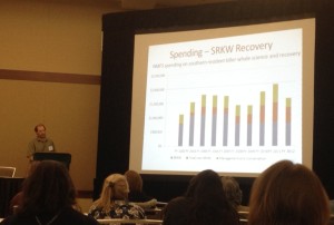
1:40 break
David Troutt, Director of Nisqually Natural Resources (for 35 years) and Chair of SRC (=Salmon Recovery Counci)
WA State salmon recovery — How we work together
2:02
State broken into regions, each with their own recovery plans (developed through the “WA way” involving many stakeholders, endorsed by Feds). Go to RCO web site for more information.
Study completed in March 2011 estimated costs of all planned regional plans is ~$5.5 billion. Funds dispersed through Salmon Recovery Funding Boards established in 1999. Funds come from PCSRF and others… Note: it is a LOT cheaper to protect than to restore…
10% of Federal grants must be used for monitoring. Example: About 80% of Nisqually outgoing smolts remain in estuary; 20% seek pocket estuaries elsewhere, but we see almost no returns of fish using the latter strategy.
There is a problem with marine survival in Puget Sound. We see 95% mortality of tagged out-going smolts between the Nisqually and Port Angeles. We’re confident that the estuary is in much better shape and 77% of the mainstem is in permanent stewardship, but we’re not seeing any result in the numbers of returning adults!
2:15 Tribal perspectives
Story: a generation of Nisqually fishers have never caught a steelhead. Annual catches of ~2k by tribes and ~2k by recreational fisheries collapsed (in 1990s?) to total run of ~500, a condition which persists. The treaties have not been withheld (and the tribes have not “shot at y’all in a long time”).
We need to work together towards ecosystem restoration. The tribes are interested in actions related to all H’s. The tribes have been working with the State to adapt how we run hatcheries to support harvest, but also be consistent with recovery goals. The North of Falcon process is part art, part science, but it is transparent and it works.
Rich Osborne, North Pacific Coast Lead Entity Coordinator (WRIA 20)
WA Sustainable Salmon Partnership — Salmon recovery on the WA coast
2:25
What’s unique about the outer coast in terms of salmon restoration?
- All 5 salmon species and steel head; none are listed except Ozette sockeye.
- Large areas are encompassed within tribal lands, which allows alternative restoration strategies.
- Almost no people! Only 7000 people on coast with no residential areas
- Large portions of watersheds in National Park, other large areas in National Forests.
Formed a non-profit to raise money beyond the SRFB: the WA Coast Sustainable Salmon Foundation. WRIA 21 = Quinalt; WRIA 22&23 Grays Harbor; WRIA 24 Pacific County.
Example projects:
- Goodman Creek road decommissioning (4 miles of road and fill removed)
- Quinalt: old logging road and fish passage blockage removal — facilitated by ability for tribe to control local decisions.
- Grays Harbor: huge estuary Chehalis has spectrum of impacts (industrial, logging, headwaters in National Park), but again not many people
- Pacific County (Willapa Bay): huge estuary w/few people; mostly Weyerhauser timber operations between pristine upper watersheds and the ocean.
28 Chinook stocks returning only 30-40,000, but could be 100s of 1000s…
An additional 12 million hatchery fish released from coastal watersheds per year
Salmon stronghold study areas (circa 2006)
 Jeannette Dormer, Puget Sound Partnership
Salmon Recovery in Puget Sound
2:45
In contrast, there are 4.1 million people in the Puget Sound region: 12 counties, 20 large cities, 100 cities total, 17 treaty tribes, many NGOs; 15 lead entities; Puget Sound Salmon Recovery Council (not the Partnership) is policy body to oversee implementation of the PS salmon recovery plan.
6 salmonid species, 3 listed under ESA (PS Chinook threatened in 1999, Hood Canal summer chum threatened in 1999, 2007 Puget Sound steelhead).
Salmon recovery success example: Puget Sound Acquisition & Restoration (PSAR) Fund. Regional priority list; increased from $15 million to $70 million appropriated for 2013-2015 biennium
- 100s of acres of estuary restoration in Snohomish and Skagit rivers
- Elwha dry lake bed reforesting
- 3+ acres eel grass on Bainbridge
- Seahurst seawall removal and restoration
Intersection with orca…
3:05
Jacque White, Exec. Director of Long Live the Kings (used to work at P4PS and Nature Conservancy)
Salish Sea marine survival project
Many partners supporting the coordinating organizations — Long Live the Kings in U.S. and Pacific Salmon Foundation in Canada
“Puget Sound salmon are sick and we don’t know why…”
- Coho marine survival declined sharply in 1980s from ~3% to <~0.5% and has persisted, while during the same period (1974-2007) WA/BC coastal survival has been fluctuating around a mean of ~0.5%. There are similar trends for steelhead and Chinook.
- Declines in Fraser sockeye, steelhead, herring spawning areas, forage fishes, hake, lingcod
- Rises in Harbor seals, lags, temperatures, and human population
- Little effort to integrate research efforts
- Now seeing economic impacts on humans (sports fishing, tribes, First Nations)
Time line:
- 2007 State of the Salmon in 2007 focused on interactions of wild and hatchery salmon
- 2012 fall workshop led to idea of a transboundary project to increase survival in the Salish Sea, improve accuracy of adult return forecasting, and assess success (or failure) of existing salmon recovery efforts.
- 2014 Comprehensive planning
- 2015+ Implementation of research
Hypotheses (trying to identify factors that control salmon and steelhead survival that can be managed)
- Bottom-up processes (PDO, environment, forage fish changes to which salmonids haven’t been able to compensate)
- Top-down (predation…)
- Other factors (toxics, disease…)
Research activities
- Focus on juvenile fish
- Predation of seals on steelhead
3:45 break
Panel discussion (audio recording: .ogg [~68 Mb] | .mp3 [~34 Mb]; responses are hard to hear for some panelists who did not use microphones)
3:58 Begin
5:14 Final comments and next steps (also included in audio recordings)
Read More
The year 2013 was an exceptionally unusual one in the world of southern resident killer whales and Pacific salmon. Most noticeably, the southern residents returned to the Salish Sea later than normal, raising concerns among conservationists. Throughout the summer, researchers and whale watch operators noted that the whales were present less than normal and the duration of their visits to the Salish Sea were abbreviated.
Meanwhile, the Chinook salmon runs on the Fraser plummeted while 80-year record returns were counted on the Columbia at the Bonneville dam fish ladder. Combined with new evidence from satellite tags that the southern residents are focused on Columbia salmon during the spring months, the sighting patterns of 2013 may indicate a transition for the urban estuary known as the Salish Sea — from one with “resident” orcas to one with southern “transient” fish-eating orcas.
Killer whale trends
Based on data from the Orca Network sighting maps from the past decade (see figure below), records were set or tied in 2013 for the least number of days spent by southern residents in the historic core of their summer habitat (the west side of San Juan Island in Haro Strait). The SRKWs were seen only once in March and not at all in April. Even more shockingly, they showed up only 5 times in May (a record low) and were observed 15 times in June, a low level not seen since 2001.

The same data show downward trends in monthly sightings over the last decade. With the exception of a high in 2011, the March prevalence has been flat or decreasing. There are stronger, more continuous downward trends in April and May sightings.

We used the OrcaMaster database maintained by The Whale Museum to look for trends in sighting “gaps” — the number of consecutive days between sightings of J pod members within the Salish Sea.  Val plotted running averages of 2013 gaps versus a historic average (1992-2012) and found that in the spring of 2013 sighting gaps were 2-5x longer than the average. Only during and after September of 2o13 did the gap return to a normal duration. (Maybe we should look at trends in Salish Sea chum run?)
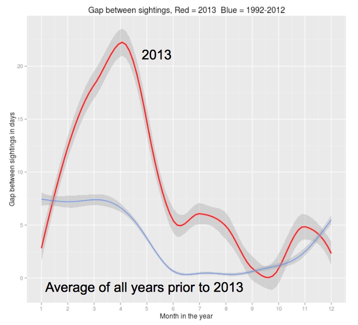
Historic trends in J pod sighting gaps (Val Veirs, using R and ggplot)
Chinook trends
One way to characterize the foraging conditions the SRKWs experienced in 2013 within the Salish Sea and on the outer coast is to examine the Chinook salmon counts from the Fraser and Columbia rivers. The Albion test fishery on the Fraser provides a proxy for the abundance of Fraser Chinook, the primary prey of SRKWs in the Salish Sea from spring through the summer (Hanson, Baird, Ford, Hempelmann-Halos, Van Doornik, Candy, Emmons, Gregory Schorr, Brian Gisborne, Katherine Ayres, Samuel Wasser, Kelley Balcomb-Bartok, John Sneva and Michael Ford, 2010). The fish counts at the Bonneville dam on the Columbia are a proxy for the abundance of Chinook on the outer coast of Washington.
As marine naturalists like Jane Cogan and Monika Wieland have pointed out, 2013 was an exceptionally bad year for Fraser Chinook returns. The fish arrived late and the cumulative returns were well below this historic average and only slightly better than in the worse year on record, 2012. The highpoint of the 2013 run was the peak around the 3rd week of August that may also be related to a pulse of Chinook recorded in the first two weeks of July off southern Vancouver Island (in the Area 20 test catch fishery).


In contrast, adult and jack Chinook abundance in the Columbia River has been on the rise for the past couple decades, with 2013 standing out as a record-setting year for adult Chinook.
 Daily Chinook counts at Bonneville show that while most of the record-setting abundance was due to the fall run, the spring run also had peaks well above the 10-year average.
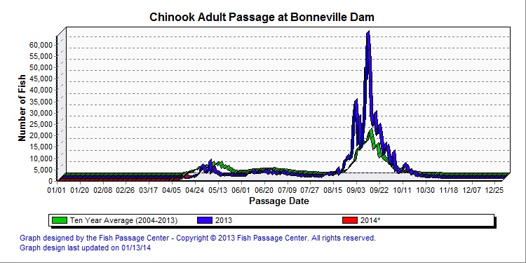
The spring run passed Bonneville from late April to late May, 2013. This timing is consistent with the timing of the spring Columbia Chinook run in 2012. Since Bonneville dam is about 200 km upstream from the river mouth and adult Chinook swim at about 0.5 m/s, we could expect that the returning Columbia Chinook were in the ocean at least until about a week before they reached Bonneville ( 200,000 m / 0.5 m/s = 400,000 seconds = ~5 days). So where were the southern residents in March and April of 2013, since they weren’t being sighted in the Salish Sea? We don’t know about J and L pods, but the satellite tag deployed on K25 indicates the likely position of K pod (up until April 4).
The answer is: during March, 2013, K25 was spending a lot of time going back and forth along the continental shelf of Washington (and to a lesser extent Oregon) with a track that centered on the mouth of the Columbia River.
We need to know more about when the returning Columbia fish are on the continental shelf and accessible to the southern resident killer whales. But these salmon trends from the region’s biggest rivers combined with migratory patterns of the orcas strongly suggest that the southern resident killer whales may be happy to move their “residence” to wherever the eating is best! Perhaps we are watching them become southern transient fish-eating killer whales?!
Anecdotal observations of orca-salmon interactions
When the fish-eaters were around during the summer of 2013, they displayed some unusually aggressive foraging. A (potential) prize Chinook salmon was taken off a derby fisherman’s line and became the focus of a KPLU radio story and an impressive photo of the one that was eaten away…
The part that didn’t get (taken) away. (credit: Kevin Klein)
This local predation event was a first for Washington State (as far as we know), though it was comparable to one by Alaskan fish-eating killer whales. In the video below, the Alaskan whales were foraging amongst fishing vessels and happened (probably visually) upon a large hooked Chinook. (Mute your speakers if you don’t want to hear angry and amazed fishermen cursing.)
Later in the summer of 2013, back in Washington, a whale watch captain obtained this video of southern resident killer whales pursuing a large (likely Chinook) salmon alongside the boat —
Could these uncommon foraging observations indicate that the southern residents were having a tough time finding enough to eat in the Salish Sea? We’d be interested in hearing from local fishers about how often they’ve had fish taken off their lines by Southern Residents. Monika assures us though that it is common to observe SRKWs pursuing salmon around and underneath whale watching boats, so maybe we should attribute the second video to more typical foraging and take it as evidence that orca-salmon interactions in the fall of 2013 were more typical than earlier in the year.
7919
{5THBC54C}
apa-no-doi-no-issue
default
ASC
no
5175
http://www.beamreach.org/wp-content/plugins/zotpress/
Hanson, M. B., Baird, R. W., Ford, J. K. B., Hempelmann-Halos, J., Van Doornik, D., Candy, J., … Michael Ford. (2010). Species and stock identification of prey consumed by endangered southern resident killer whales in their summer range. Endangered Species Research, 11, 69–82.
Read More
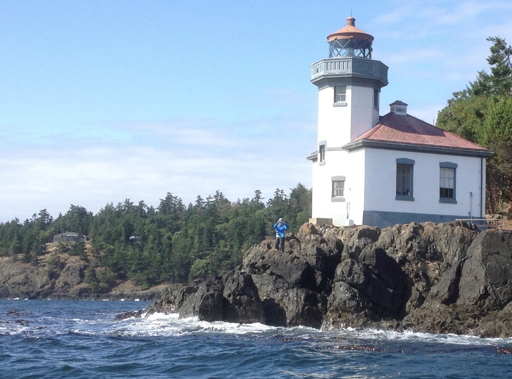

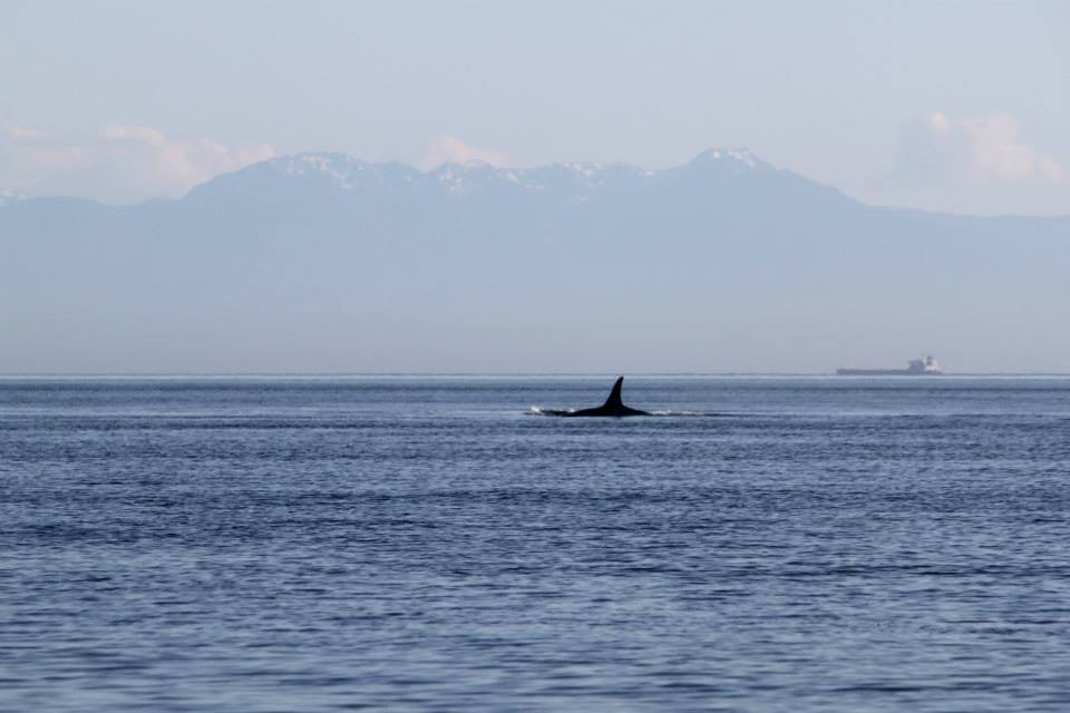
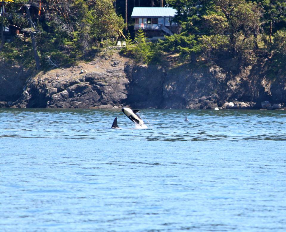

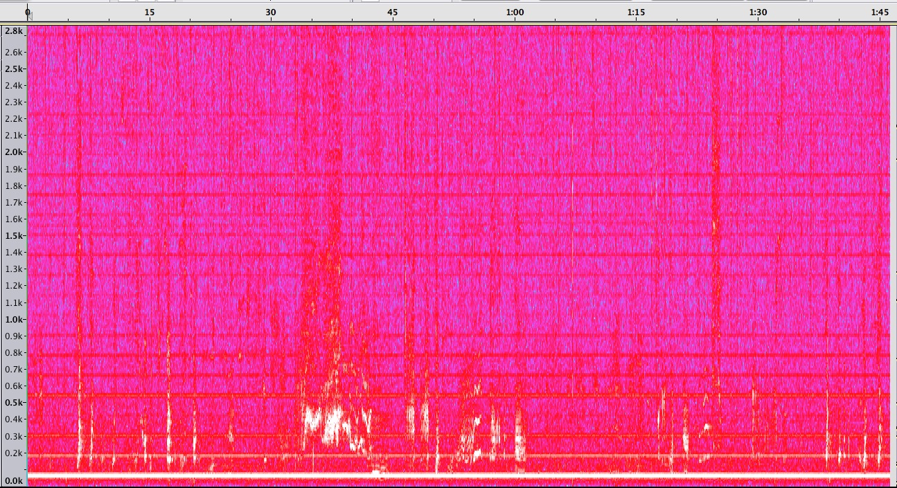

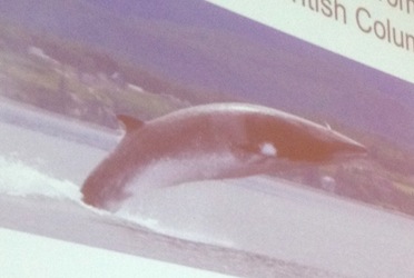


 Twitter
 LinkedIn
 Facebook